Visualización Computacional II

Presentación del tema: "Visualización Computacional II"— Transcripción de la presentación:

1 Visualización Computacional II

2 Edificio PLADEMA Quienes somos? Profesor: Ayudantes:
Dr. Marcelo Javier Vénere: Ayudantes: Ing. Juan P. D’Amato: Ing. Cristian García Bauza: Edificio PLADEMA

3 Logística (o como va a ser la cosa…)
Seis clases teóricas repartidas entre esta semana y la que viene. Dos prácticas (a confirmar) para explicación de conceptos (OpenGL) y uso de tutoriales. Tres prácticas adicionales Forma de evaluación: Cursada y Final con un trabajo. Una entrega a corto plazo (antes de fin de año) y entrega final posterior.

4 Horarios y Lugares Teórica: Martes 21/10: Aula 2 (Facultad) 19-22 hs.
Miércoles 22/10: Aula 2 (Facultad) hs. Viernes 24/10: Aula 1 (Facultad) hs. Lunes 27/10: Aula 3 (Facultad) hs. Martes 28/10: Aula 2 (Facultad) hs. Miércoles 29/10: A confirmar

5 Información Bibliografía:
Foley, van Dam, Feiner, Hughes “Computer Graphics: Principles and Practice”. Woo, Neider, Davis, Shreiner: “OpenGL Programming Guide”. Alan Watt “3D Computer Graphics”. IEEE Computer Graphics an applications.

6 Objetivo Idea: Entender los principios y metodologías para lograr efectos especiales en aplicaciones 3D.

7 Resumen de la materia Iluminación y transformaciones. Texturas.
Raycasting, Raytracing y Radiosity. Sombras. Animación y comportamiento físico. Optimizaciones.

8 Transformaciones Las transformaciones se aplican sobre
los puntos que definen el objeto Pi P1 P2 Pi = (px, py)

9 Transformaciones Simples
Escala isotrópica Pi = (px, py) sx 0 0 sy S = Pi = S.Pi

10 Transformaciones Simples
Traslación dx dy Pi = Pi + D Pi = (px, py) D = (dx, dy)

11 Transformaciones Simples
Rotación Pi = (px, py) cos  -sin  sin  cos  R = Pi = R.Pi  

12 Como representar las transformaciones?
x' = ax + by + c y' = dx + ey + f x' y' a b d e x y c f = + p' = M p t

13 Coordenadas homogeneas
Se agrega una dimensión extra en 2D, se usa 3 x 3 matrices en 3D, se usa 4 x 4 matrices Cada punto tiene entonces un valor extra, w x' y' z' w' a e i m b f j n c g k o d h l p x y z w = p' = M p

14 Pasar a coordenadas homogeneas
x' = ax + by + c y' = dx + ey + f Forma Afín Forma Homogénea x' y‘ 1 a b d e 0 0 c f 1 x y 1 x' y' a b d e x y c f = = + p' = M p t p' = M p

15 Traslación (tx, ty, tz) x' y' z' 1 x' y' z' 1 1 1 tx ty tz 1 x y z 1 =
Por que utilizar coordenadas homogéneas? Porque ahora las traslaciones se expresan como matriz! x' y' z' 1 x' y' z' 1 1 1 tx ty tz 1 x y z 1 =

16 Escala (sx, sy, sz) x' y' z' 1 sx sy sz 1 x y z 1 = Scale(s,s,s)
p' p Isotrópica (uniforme) scaling: sx = sy = sz q' q x x' y' z' 1 sx sy sz 1 x y z 1 =

17 Rotación x' y' z' 1 cos θ sin θ -sin θ cos θ 1 1 x y z 1 = ZRotate(θ)
p' Sobre eje z θ p x z x' y' z' 1 cos θ sin θ -sin θ cos θ 1 1 x y z 1 =

18 V’ = R . V Rotación x' y' z' 1 r11 r21 r31 r12 r22 r32 r13 r23 r33 1 x
General x' y' z' 1 r11 r21 r31 r12 r22 r32 r13 r23 r33 1 x y z 1 = V’ = R . V

19 Proyección en perspectiva
x' y' z' w’ 1 1 1 1/d x y z 1 = V’ = P. R . V

20 Necesidad de un modelo de iluminación

21 Difusor perfecto I R = I.Kr G = I.Kg B = I.Kb
Asumimos que la superficie refleja igual en todas las direcciones. Ejemplo: tiza, arcilla, algunas pinturas R = I.Kr G = I.Kg B = I.Kb I Superficie

22 Cantidad de luz recibida
Surface  n I0 I = I0.cos  R = I0.cos .Kr G = I0.cos .Kg B = I0.cos .Kb

23 Reflejos Reflexión ocurre solo en la dirección especular. n   r l
Depende de la posición relativa de la fuente de luz y el punto de vista A second surface type is called a specular reflector. When we look at a shiny surface, such as polished metal or a glossy car finish, we see a highlight, or bright spot. Where this bright spot appears on the surface is a function of where the surface is seen from. This type of reflectance is view dependent. At the microscopic level a specular reflecting surface is very smooth, and usually these microscopic surface elements are oriented in the same direction as the surface itself. Specular reflection is merely the mirror reflection of the light source in a surface. Thus it should come as no surprise that it is viewer dependent, since if you stood in front of a mirror and placed your finger over the reflection of a light, you would expect that you could reposition your head to look around your finger and see the light again. An ideal mirror is a purely specular reflector. In order to model specular reflection we need to understand the physics of reflection. n   r l Surface

24 Reflectores no ideales
Materiales reales no son como espejos. Brillos no son puntuales sino borrosos At this point we will introduce an empirical model that is consistent with our experience, at least to a crude approximation. In general, we expect most of the reflected light to travel in the direction of the ideal ray. However, because of microscopic surface variations we might expect some of the light to be reflected just slightly offset from the ideal reflected ray. As we move farther and farther, in the angular sense, from the reflected ray we expect to see less light reflected.

25 Reflectores no ideales
Modelo empírico simple: Se supone que la luz se reflejará en la dirección del rayo ideal. Sin embargo, debido a imperfecciones microscópicas de la superficie, algunos rayos reflejados se apartarán un poco de la dirección ideal.

26 El modelo Phong I = I0.Ks.cosq Parámetros n r   L Cámara  V
ks: coeficiente reflexión especular q : exponente reflexión especular I = I0.Ks.cosq n r One function that approximates this fall off is called the Phong Illumination model. This model has no physical basis, yet it is one of the most commonly used illumination models in computer graphics. The cosine term is maximum when the surface is viewed from the mirror direction and falls off to 0 when viewed at 90 degrees away from it. The scalar nshiny controls the rate of this fall off.   L Cámara  V Surface

27 El modelo Phong Efecto del coeficiente q
The diagram below shows the how the reflectance drops off in a Phong illumination model. For a large value of the nshiny coefficient, the reflectance decreases rapidly with increasing viewing angle.

28 Cálculo de la dirección especular
R = I0.((1-Ks).Kr. L.n + Ks. (V.r)q) G = I0.((1-Ks).Kg. L.n + Ks. (V.r)q) B = I0.((1-Ks).Kb. L.n + Ks. (V.r)q) r   L r Surface

29 Modelo de iluminación simple
R =Ia.Kr + I0.((1-Ks).Kr. L.n + Ks. (V.r)q) G = Ia.Kg + I0.((1-Ks).Kg. L.n + Ks. (V.r)q) B = Ia.Kb + I0.((1-Ks).Kb. L.n + Ks. (V.r)q) Surface

30 Modelos de iluminación (resumen)
R = Ia.Kr + Σ Ii.((1-Ks).Kr. Li.n + Ks. (V.ri)q) G = Ia.Kg + Σ Ii.((1-Ks).Kg. Li.n + Ks. (V.ri)q) B = Ia.Kb + Σ Ii.((1-Ks).Kb. Li.n + Ks. (V.ri)q) L Kr, Kg, Kb Ks, q Propiedades del cuerpo r n V Surface

31 Intensidad de la luz En realidad se usa 1/r Decae como 1/r2
Misma energía en todas las direcciones En realidad se usa 1/r

32 Modelo de iluminación simple
Flat shading Gourard shading

33 Gourard shading n1 , n2 , n3 Ir1 , Ig1 , Ib1 Ir2 , Ig2 , Ib2
Irpixel= (Ir1.A1+Ir2.A2+Ir3.A3)/A

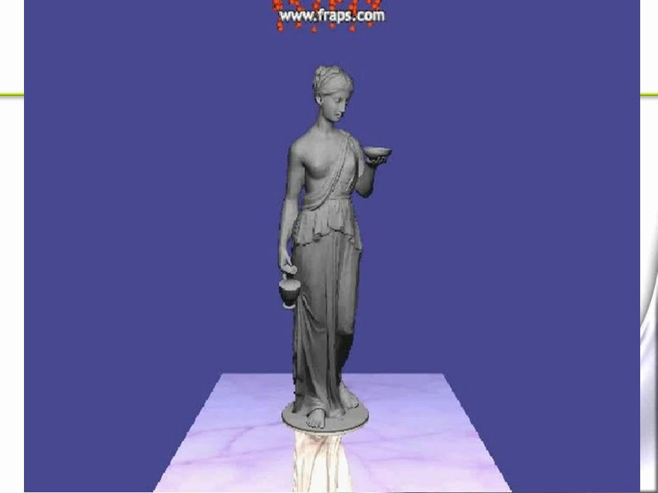
34 Phong shading n1 , n2 , n3 npixel Ir , Ig , Ib

35 Modelo de iluminación simple

36 Modelo de iluminación simple

37 Que falta tener en cuenta?
Para obtener imágenes realistas Texturas Sombras Transparencias Reflexiones Refracciones Fuentes no puntuales Iluminación proveniente de otros objetos

38 Resumen - Texturas Por qué usar texturas Conceptos básicos
Mapeo y Tiling Filtros y Mipmapping Lightmaps y efectos. Environment Mapping

39 Resumen - Sombras Fake shadows Planar & Projective Shadow Mapping
Shadow volumes

40 Transparencias

41 Refracción

42 Reflexiones

43 Ray Tracing I = Ilocal + Ireflejada + Irefractada

44 Sombras difusas

45 Radiosity

46

47

48 Que falta tener en cuenta?
Para lograr realidad virtual Inmersión Comportamientos realistas Matrix

49 Efectos físicos

50 Efectos físicos

51

52