Descargar la presentación
La descarga está en progreso. Por favor, espere

1
3 er Máster “Cambio global” (Palma de Mallorca, octubre de 2010) Módulo 2.02: “Consecuencias hidrológicas y biogeoquímicas del Cambio Global en los ecosistemas continentales” Tema 18: “Ciclo global contemporáneo del carbono y cambios bajo un escenario de cambio climático” Juan Carlos Rodríguez Murillo, científico titular, IRN-CCMA, CSIC
 Módulo 2.02: Consecuencias hidrológicas y biogeoquímicas del Cambio Global en los ecosistemas continentales Tema 18: Ciclo global contemporáneo del carbono y cambios bajo un escenario de cambio climático Juan Carlos Rodríguez Murillo, científico titular, IRN-CCMA, CSIC")
2
El ciclo global del carbono The global carbon cycle 1)Introducción /Introduction 2) Descripción general del ciclo del carbono / General description of carbon cycle 3) Depósitos del ciclo (rápido) del carbono / Reservoirs of the (fast) carbon cycle 4) Impactos del cambio global en el ciclo del carbono / Global change impacts on carbon cycle 5) Métodos de estimación de depósitos y flujos de carbono / Methods of estimation of reservoir and carbon fluxes
Introducción /Introduction 2) Descripción general del ciclo del carbono / General description of carbon cycle 3) Depósitos del ciclo (rápido) del carbono / Reservoirs of the (fast) carbon cycle 4) Impactos del cambio global en el ciclo del carbono / Global change impacts on carbon cycle 5) Métodos de estimación de depósitos y flujos de carbono / Methods of estimation of reservoir and carbon fluxes")
3
El carbono en la Tierra / Carbon on Earth Es el elemento clave de los seres vivos. / Carbon is the key element for living beings El ciclo del carbono incluye al carbono orgánico en todas sus formas (la totalidad de los seres vivos y de las moléculas orgánicas), así como al C inorgánico, fundamentalmente en forma de CO, CO 2 y (bi) carbonatos. / Carbon cycle includes organic carbon in all forms (all the living beings and organic molecules), as well as inorganic carbon, mostly as CO, CO 2 and (bi) carbonates Los flujos de carbono en el ciclo están asociados a procesos bioquímicos (fotosíntesis y respiración), físicoquímicos (disolución de CO 2 en el agua), químicos (meteorización de silicatos, disolución y precipitación de carbonatos) y físicos (erosión, transporte y deposición). / Carbon fluxes are associated to biochemical (photosynthesis and respiration), physicochemical (CO 2 dissolution in water), chemical (silicate weathering, carbonate dissolution and precipitation) and physical (erosion, transport, and deposition) 1)Introducción
, así como al C inorgánico, fundamentalmente en forma de CO, CO 2 y (bi) carbonatos. / Carbon cycle includes organic carbon in all forms (all the living beings and organic molecules), as well as inorganic carbon, mostly as CO, CO 2 and (bi) carbonates Los flujos de carbono en el ciclo están asociados a procesos bioquímicos (fotosíntesis y respiración), físicoquímicos (disolución de CO 2 en el agua), químicos (meteorización de silicatos, disolución y precipitación de carbonatos) y físicos (erosión, transporte y deposición). / Carbon fluxes are associated to biochemical (photosynthesis and respiration), physicochemical (CO 2 dissolution in water), chemical (silicate weathering, carbonate dissolution and precipitation) and physical (erosion, transport, and deposition) 1)Introducción.")
4
El carbono en la Tierra/ Carbon on Earth El compuesto fundamental del ciclo del carbono es el dióxido de carbono (CO 2 )./ CO 2 is the basic compound in the carbon cycle Este gas es prácticamente inerte en la atmósfera, pero soluble en el agua, y materia prima de la fotosíntesis y producto de la respiración./ CO 2 is practically inert in the atmosphere, but is water soluble, and is the photosynthesis raw material, as well as a main product of respiration Por ello, el CO 2 es el componente fundamental de los flujos de C entre la atmósfera y la biosfera y la atmósfera y los océanos. /Therefore, CO 2 is the main compound in biosphere-atmosphere and ocean-atmosphere C fluxes Además, por su participación en la meteorización de los silicatos y en la disolución y precipitación de carbonatos, contribuye al reciclado de volátiles a través de la litosfera y forma las rocas sedimentarias carbonatadas. Aditionally, CO 2 contributes to volatile recycling through lithosphere, and produces sedimentary limestones by its role in silicate weathering and carbonate dissolution and precipitation, respectively.

5
2) Descripción general del ciclo del carbono / General description of carbon cycle
 Descripción general del ciclo del carbono / General description of carbon cycle")
7
El CO 2 atmosférico es estable químicamente. Su vida media atmosférica es de 750 Gt/(120 + 92 Gt año-1) ó 3,5 años, antes de entrar en los ecosistemas terrestres o en los océanos. / Atmospheric CO 2 is chemically stable, with an average atmospheric lifetime of 3.5 years, before entering terrestrial ecosystems or oceans. O Flujos atmósfera-tierra: - Fotosíntesis (CO 2 + H 2 O CH 2 O + O 2 ) - Respiración (oxidación) O HCO 3 - + H + Flujos atmósfera-océano: - Disolución de CO 2 (CO 2 + H 2 O HCO 3 - + H + HCO 3 - CO 3 -2 + H + HCO 3 - CO 3 -2 + H + - Desgasificación de - Desgasificación de CO 2
 ó 3,5 años, antes de entrar en los ecosistemas terrestres o en los océanos. / Atmospheric CO 2 is chemically stable, with an average atmospheric lifetime of 3.5 years, before entering terrestrial ecosystems or oceans. O Flujos atmósfera-tierra: - Fotosíntesis (CO 2 + H 2 O CH 2 O + O 2 ) - Respiración (oxidación) O HCO H + Flujos atmósfera-océano: - Disolución de CO 2 (CO 2 + H 2 O HCO H + HCO 3 - CO H + HCO 3 - CO H + - Desgasificación de - Desgasificación de CO 2.")
8
Ciclos del carbono “rápido” y “lento”/ “Slow” and “fast “ carbon cycles En estado estacionario, el tiempo de residencia del C en cada depósito será = (Tamaño del depósito/flujo de salida). /Admitting steady-state, C turnover in each reservoir is = (Reservoir size / Output flux) Los depósitos geológicos de C (carbonatos de los sedimentos y C orgánico en forma de querógeno o combustibles fósiles) tienen tiempos de residencia de cientos de millones de años. / C turnover in geological reservoirs (sedimentary limestone and organic C as kerogen) takes hundreds of million years Los depósitos de C atmosférico, biosférico y oceánico superficial intercambian C en años o decenas de años. / Atmospheric, biospheric and shallow sea reservoirs have turnover times of years or tens of years El C tiene unos 500 años de tiempo de residencia en el depósito oceánico total. / Turnover of C in the whole ocean takes about 500 years
 Los depósitos geológicos de C (carbonatos de los sedimentos y C orgánico en forma de querógeno o combustibles fósiles) tienen tiempos de residencia de cientos de millones de años. / C turnover in geological reservoirs (sedimentary limestone and organic C as kerogen) takes hundreds of million years Los depósitos de C atmosférico, biosférico y oceánico superficial intercambian C en años o decenas de años. / Atmospheric, biospheric and shallow sea reservoirs have turnover times of years or tens of years El C tiene unos 500 años de tiempo de residencia en el depósito oceánico total. / Turnover of C in the whole ocean takes about 500 years.")
9
Podemos, pues, distinguir un ciclo lento geológico, de flujos lentos que determinan la concentración atmosférica del CO 2 a escalas de millones de años, y un ciclo rápido biogeoquímico, que influye en dicha concentración a escala de decenios-centenas de años. /We may differentiate a geological slow cycle, made of slow fluxes which determine the atmospheric CO 2 concentration in the million-year range, and a biogeochemical fast cycle, which establishes CO 2 concentration in the short term (decade – centennial)
.")
10
Otros procesos del ciclo del carbono / Other processes in the carbon cycle - Procesos del ciclo geológico del carbono / Processes in carbon geological cycle 1) Meteorización de silicatos: CaSiO 3 + 2CO 2 + H 2 O Ca 2+ + 2HCO 3 +SiO 2 2) Precipitación/disolución de carbonatos: Ca 2+ + 2HCO 3 CaCO 3 + CO 2 + H 2 O 3) Metamorfismo: CaCO 3 + SiO 2 CaSiO 3 + CO 2 - Procesos del subciclo del metano /Methane subcycle processes
 Meteorización de silicatos: CaSiO 3 + 2CO 2 + H 2 O Ca HCO 3 +SiO 2 2) Precipitación/disolución de carbonatos: Ca HCO 3 CaCO 3 + CO 2 + H 2 O 3) Metamorfismo: CaCO 3 + SiO 2 CaSiO 3 + CO 2 - Procesos del subciclo del metano /Methane subcycle processes")
11
Figure 1. Cartoon of fluxes (arrows) and inventories (number in boxes) of the labile components of the global carbon system for the 1980's. The red arrows are the perturbation fluxes resulting from emissions of anthropogenic CO 2. From Sabine et al. (2003).
 and inventories (number in boxes) of the labile components of the global carbon system for the 1980 s. The red arrows are the perturbation fluxes resulting from emissions of anthropogenic CO 2. From Sabine et al. (2003)..")
12
El subciclo del metano / The methane subcycle Dentro del ciclo del carbono, “movido” mayoritariamente por el CO 2, podemos distinguir un subciclo, cuyo componente dinámico es el metano (CH 4 ). / As a part of C cycle, one can analyze a methane (CH 4 ) subcycle El metano es la “parte anaerobia” del ciclo del carbono, ya que su producción requiere la ausencia de oxígeno./ Methane represents the “anaerobic side” of carbon cycle, because its production needs oxygen absence
 subcycle El metano es la parte anaerobia del ciclo del carbono, ya que su producción requiere la ausencia de oxígeno./ Methane represents the anaerobic side of carbon cycle, because its production needs oxygen absence.")
13
La generación de metano se produce en el metabolismo de diferentes procariotas (bacterias metanogénicas) por descomposición del acetato (dando CO 2 como subproducto) o por reducción del CO 2 con H 2 (reducción disimilatoria de CO 2 )./ Methane generation occurs in methanogenic bacteria metabolism, by acetate decomposition (giving CO 2 as byproduct) or by H 2 mediated CO 2 reduction (dissimilatory CO 2 reduction) El consumo de metano se produce también por oxidación con O 2 en bacterias (metanotróficas), por oxidación con sulfato (bacterias sulfato- reductoras), y por oxidación atmosférica con el radical hidroxilo./ Methane consumption occurs by O 2 oxidation in bacteria (methanotrophic), by oxidation with sulfate (sulfate-reducing bacteria), and by atmospheric oxidation with hydroxyl radical. Generación / descomposición de metano

16
Atmosphere Fossil Deposits 6.3 63.0 91.7 60 90 3.2 Plants Soil Oceans 750 500 2000 38,400 About 4,100 1.6 Units Gt C Gt C y -1 0.7 3) DEPÓSITOS DEL CICLO (RÁPIDO) DEL CARBONO /Reservoirs of the (fast) carbon cycle
 DEPÓSITOS DEL CICLO (RÁPIDO) DEL CARBONO /Reservoirs of the (fast) carbon cycle")
17
LA ATMÓSFERA

18
La atmósfera primitiva y la actual / Primeval and present atmosphere Las masas de agua, C, N y S en la superficie terrestre actual son casi las mismas de las de los compuestos volátiles que constituían la atmósfera de la Tierra primitiva./ Masses of water, C, N, and S on the present Earth surface are almost equal to those of the volatile compounds which made up the primitive Earth atmosphere La atmósfera primitiva procedente de la desgasificación de estos compuestos volátiles contenía agua (90%) y CO 2 (7-8%), con algo de N 2, HCl y H 2 S./ Primeval atmosphere from volatilization of these volatile compounds contained water (90%) and CO 2 (7-8%), with minor quantities of N 2, HCl y H 2 S Al enfriarse la Tierra, el agua se condensó, disolviendo a todos los volátiles menos el N 2. La atmósfera quedó formada por nitrógeno y CO 2./ As Earth cooled, water condensed, dissolving volatiles except N 2. Only CO 2 and N remained in the atmosphere La concentración atmosférica de CO 2 en el Precámbrico fue disminuyendo por formación de carbonatos y de materia orgánica./ The CO 2 atmospheric concentration in Precambric was falling by carbonate and organic matter formation

19
El CO 2 a través de la historia geológica Aumento de CO 2 : Desgasificación (vulcanismo, tectónica). Disminución de CO 2 : Meteorización, depósitos de materia orgánica).
..")
20
El CO 2 a través de la historia geológica: El Pleistoceno

21
El CO 2 reciente

22
El CO 2 reciente y en un futuro cercano

23
-Variación reciente de CO 2 y oxígeno. - Emisiones antrópicas de C y variación de δ 13 C.

24
Figure 2.3. Recent CO2 concentrations and emissions. (a) CO2 concentrations (monthly averages) measured by continuous analysers over the period 1970 to 2005 from Mauna Loa, Hawaii (19°N, black; Keeling and Whorf, 2005) and Baring Head, New Zealand (41°S, blue; following techniques by Manning et al., 1997). Due to the larger amount of terrestrial biosphere in the NH, seasonal cycles in CO2 are larger there than in the SH. In the lower right of the panel, atmospheric oxygen (O2) measurements from fl ask samples are shown from Alert, Canada (82°N, pink) and Cape Grim, Australia (41°S, cyan) (Manning and Keeling, 2006). The O2 oncentration is measured as ‘per meg’ deviations in the O2/N2 ratio from an arbitrary reference,analogous to the ‘per mil’ unit typically used in stable isotope work, but where the ratio is multiplied by 106 instead of 103 because much smaller changes are measured. (b) Annual global CO2 emissions from fossil fuel burning and cement manufacture in GtC yr–1 (black) through 2005, using data from the CDIAC website (Marland et al, 2006) to 2003. Emissions data for 2004 and 2005 are extrapolated from CDIAC using data from the BP Statistical Review of World Energy (BP, 2006). Land use emissions are not shown; these are estimated to be between 0.5 and 2.7 GtC yr–1 for the 1990s (Table 7.2). Annual averages of the 13C/12C ratio measured in atmospheric CO2 at Mauna Loa from 1981 to 2002 (red) are also shown (Keeling et al, 2005). The isotope data are expressed as δ13C(CO2) ‰ (per mil) deviation from a calibration standard. Note that this scale is inverted to improve clarity.
 CO2 concentrations (monthly averages) measured by continuous analysers over the period 1970 to 2005 from Mauna Loa, Hawaii (19°N, black; Keeling and Whorf, 2005) and Baring Head, New Zealand (41°S, blue; following techniques by Manning et al., 1997). Due to the larger amount of terrestrial biosphere in the NH, seasonal cycles in CO2 are larger there than in the SH. In the lower right of the panel, atmospheric oxygen (O2) measurements from fl ask samples are shown from Alert, Canada (82°N, pink) and Cape Grim, Australia (41°S, cyan) (Manning and Keeling, 2006). The O2 oncentration is measured as ‘per meg’ deviations in the O2/N2 ratio from an arbitrary reference,analogous to the ‘per mil’ unit typically used in stable isotope work, but where the ratio is multiplied by 106 instead of 103 because much smaller changes are measured. (b) Annual global CO2 emissions from fossil fuel burning and cement manufacture in GtC yr–1 (black) through 2005, using data from the CDIAC website (Marland et al, 2006) to Emissions data for 2004 and 2005 are extrapolated from CDIAC using data from the BP Statistical Review of World Energy (BP, 2006). Land use emissions are not shown; these are estimated to be between 0.5 and 2.7 GtC yr–1 for the 1990s (Table 7.2). Annual averages of the 13C/12C ratio measured in atmospheric CO2 at Mauna Loa from 1981 to 2002 (red) are also shown (Keeling et al, 2005). The isotope data are expressed as δ13C(CO2) ‰ (per mil) deviation from a calibration standard. Note that this scale is inverted to improve clarity..")
25
El metano atmosférico reciente No se conoce la razón de la estabilización del metano en la atmósfera, aunque parece deberse a la disminución de las fuentes. Recientemente (2007), el metano parece aumentar./ Reasons for atmospheric methane concentration levelling off are not known, but a source decrease is the probable cause. Recently (2007), methane seems to increase again
, el metano parece aumentar./ Reasons for atmospheric methane concentration levelling off are not known, but a source decrease is the probable cause. Recently (2007), methane seems to increase again.")
26
LOS OCÉANOS

27
Los océanos : Cambios en el dióxido de carbono disuelto/ Oceans: Changes in dissolved carbon dioxide

30
LOS ECOSISTEMAS TERRESTRES

31
Table 1: Global carbon stocks in vegetation and soil carbon pools down to a depth of 1 m. Biome Area (10 9 ha) Global Carbon Stocks (Gt C) VegetationSoilTotal Tropical forests1.76212216428 Temperate forests1.0459100159 Boreal forests1.3788471559 Tropical savannas2.2566264330 Temperate grasslands1.259295304 Deserts and semideserts4.558191199 Tundra0.956121127 Wetlands0.3515225240 Croplands1.603128131 Total15.1246620112477 Note: There is considerable uncertainty in the numbers given, because of ambiguity of definitions of biomes, but the table still provides an overview of the magnitude of carbon stocks in terrestrial systems.
 Global Carbon Stocks (Gt C) VegetationSoilTotal Tropical forests Temperate forests Boreal forests Tropical savannas Temperate grasslands Deserts and semideserts Tundra Wetlands Croplands Total Note: There is considerable uncertainty in the numbers given, because of ambiguity of definitions of biomes, but the table still provides an overview of the magnitude of carbon stocks in terrestrial systems..")
32
Total C en vegetación: 466 Gt Total C en suelos: 2.011 Gt (IPCC, 2000, “Land use, land-use change and forestry”)
")
33
Los ecosistemas terrestres Global terrestrial carbon uptake was simulated by 11 coupled carbon-cycle–climate models driven with carbon emissions from the SRES-A2 emissions profile. Data are taken from the Coupled Carbon Cycle Climate Model Intercomparison Project 2, with uptake rates smoothed with a 30-year moving average. 2 Nature 451, 289-292 (17 January 2008) | Terrestrial ecosystem carbon dynamics and climate feedbacks Martin Heimann 1 & Markus Reichstein 1 1
 | Terrestrial ecosystem carbon dynamics and climate feedbacks Martin Heimann 1 & Markus Reichstein 1 1.")
34
4) Impactos del cambio global en el ciclo del carbono / Global change impacts on carbon cycle
 Impactos del cambio global en el ciclo del carbono / Global change impacts on carbon cycle")
36
(Woods Hole Research Center)
")
37
Las variaciones de la tasa de crecimiento de la concentración atmosférica de CO 2 están causadas principalmente por efectos terrestres, particularmente por los impactos de las olas de calor y las sequías en la vegetación de la Amazonía occidental y del sudeste asiático, que producen pérdidas de C en los ecosistemas debido a la menor productividad vegetal y/o incremento de la respiración. / Fluctuations of atmospheric CO 2 concentration growth rate are mainly the result of terrestrial effects, particularly of heathwave and drought impacts on Western Amazonia and Southeastern Asia vegetation, which cause a loss of ecosystem carbon due to lower plant production and/or increased respiration

38
Inferred changes in CO 2 flux compared with the 1980- 98 mean Bousquet et al (2000) Science 290 1342 Land Oceans ̃
 Science Land Oceans ̃")
39
Balance moderno de carbono: CF – A CF: Flujo por combustibles fósiles y cemento A: Aumento atmosférico de C Gran sumidero oceánico y sumidero variable en la biosfera. /Modern C budget: Big ocean sink and variable biospheric sink. Budget is = CF –A, CF being the C flux from fossil fuels and A the atmospheric C growth. Balance preindustrial de carbono: Casi en equilibrio (cambios lentos en el CO 2 atm.) Pequeña fuente en el océano. /Preindustrial C budget: Near equilibrium. Slow changes in atmospheric CO 2. Small oceanic source Los flujos CF y A están muy bien caracterizados. La diferencia CF – A se ha de repartir entre la biosfera y el océano. Este reparto varía temporalmente y espacialmente. / CF and A fluxes are very well determined. CF –A must be shared between biosphere and ocean. Shares vary temporally and spatially. El sumidero oceánico está bien relativamente bien caracterizado:/ Ocean sink is relatively well characterized - Por los modelos de circulación oceánica./ By ocean circulation models -Por las medidas de la evolución temporal del 13 C./ By 13 C temporal evolution measurements - Por las medidas de la evolución temporal del O 2./ By O 2 temporal evolution measurements Los océanos absorben CO 2 a altas latitudes (formación de aguas profundas –debido al downwelling- y lo emiten a bajas latitudes (por el upwelling) / Oceans absorb CO 2 at high latitudes (by downwelling) and emit at low latitudes (by upwelling)
 Pequeña fuente en el océano. /Preindustrial C budget: Near equilibrium. Slow changes in atmospheric CO 2. Small oceanic source Los flujos CF y A están muy bien caracterizados. La diferencia CF – A se ha de repartir entre la biosfera y el océano. Este reparto varía temporalmente y espacialmente. / CF and A fluxes are very well determined. CF –A must be shared between biosphere and ocean. Shares vary temporally and spatially. El sumidero oceánico está bien relativamente bien caracterizado:/ Ocean sink is relatively well characterized - Por los modelos de circulación oceánica./ By ocean circulation models -Por las medidas de la evolución temporal del 13 C./ By 13 C temporal evolution measurements - Por las medidas de la evolución temporal del O 2./ By O 2 temporal evolution measurements Los océanos absorben CO 2 a altas latitudes (formación de aguas profundas –debido al downwelling- y lo emiten a bajas latitudes (por el upwelling) / Oceans absorb CO 2 at high latitudes (by downwelling) and emit at low latitudes (by upwelling).")
40
Balance mundial del carbono/ Global carbon budget 1980s1990s Incremento atmosférico 3,3 ± 0.1 3,2 ± 0.1 Emisiones “fósiles” 5,4 ± 0.3 6,3 ± 0.4 Flujo océano - atmósfera -1,8 ± 0.8 -2,1 ± 0.7 Flujo tierra – atmósfera -0,3 ± 0,9 -1,0 ± 0,8 Flujo por cambios de uso 0,9 a 2,8 1,4 a 3,0 Flujo residual terrestre -4,0 a -0,3 -4,8 a -1,6 El sumidero terrestre de carbono parece intensificarse / The terrestrial carbon sink seems to increase

41
Balance mundial del carbono por zonas (años 90)/ Global C budget by zones (90’) Total: -0,7 ± 0,8 Gt C Hemisferio Norte excepto trópico: -2,1 ± 0,8 Gt C Hemisferio Sur excepto trópico: -0,2 Gt C Trópicos : + 1,5 ± 1,2 Gt C Es decir, que existiría un sumidero terrestre de C en latitudes altas (especialmente en el hemisferio N), y una fuente en bajas latitudes./ There is a terrestrial C sink at high latitudes (mainly in N hemisphere), and a source at low latitudes.
/ Global C budget by zones (90’) Total: -0,7 ± 0,8 Gt C Hemisferio Norte excepto trópico: -2,1 ± 0,8 Gt C Hemisferio Sur excepto trópico: -0,2 Gt C Trópicos : + 1,5 ± 1,2 Gt C Es decir, que existiría un sumidero terrestre de C en latitudes altas (especialmente en el hemisferio N), y una fuente en bajas latitudes./ There is a terrestrial C sink at high latitudes (mainly in N hemisphere), and a source at low latitudes.")
42
Balance mundial del carbono/ Global carbon budget (2000-2005) Incremento atmosférico 4,3 Emisiones “fósiles” 7,2 Flujo océano - atmósfera -2,3 Flujo tierra – atmósfera -0,6 Flujo por cambios de uso 1,5 Flujo residual terrestre -2,1 Se acelera la acumulación atmosférica de carbono / Atmospheric C accumulation increases Se intensifica el sumidero oceánico / Oceanic sink intensifies Se reduce el sumidero terrestre ? / Is terrestrial sink getting smaller?

43
Mecanismos propuestos para el sumidero terrestre de C/ Proposed mechanisms for terrestrial C sink Mecanismos fisiológicos: /Physiological mechanisms: -Fertilización con CO 2 / CO 2 fertilization -Fertilización con N / N fertilization - Cambios de clima (T, humedad) / Climate changes (T, humidity) Mecanismos ecosistémicos:/ Ecosystemic mechanisms -Recrecimiento forestal tras perturbaciones humanas./ Forest regrowth following human perturbation -Menor deforestación./ Lower deforestation - Supresión de incendios e “invasión” de matorrales./ Fire supression and bush encroachment - Mejores prácticas agrícolas./ Better agricultural practices - Productos forestales y vertederos./ Forest products and landfills - Erosión y deposición de sedimentos./ Sediment erosion and deposition
 / Climate changes (T, humidity) Mecanismos ecosistémicos:/ Ecosystemic mechanisms -Recrecimiento forestal tras perturbaciones humanas./ Forest regrowth following human perturbation -Menor deforestación./ Lower deforestation - Supresión de incendios e invasión de matorrales./ Fire supression and bush encroachment - Mejores prácticas agrícolas./ Better agricultural practices - Productos forestales y vertederos./ Forest products and landfills - Erosión y deposición de sedimentos./ Sediment erosion and deposition")
44
Problemas para identificar y cuantificar los mecanismos de acumulación de carbono / Problems to identify and quantify carbon sequestration mechanisms Dificultad en determinar pequeñas variaciones de un gran sumidero (en especial, de los suelos)./ Difficulties to determine small changes in a big sink (specially soils) Dificultad en extrapolar los resultados de experiencias a pequeña escala hasta mayores escalas./ Difficulties to extrapolate small-scale experiences to bigger scales Deficiente representación en los modelos biosféricos de los procesos ecológicos relevantes para el ciclo del carbono./ Poor representation of carbon cycle relevant ecological processes in current biospherical models
./ Difficulties to determine small changes in a big sink (specially soils) Dificultad en extrapolar los resultados de experiencias a pequeña escala hasta mayores escalas./ Difficulties to extrapolate small-scale experiences to bigger scales Deficiente representación en los modelos biosféricos de los procesos ecológicos relevantes para el ciclo del carbono./ Poor representation of carbon cycle relevant ecological processes in current biospherical models")
45
¿Qué factores son más importantes en determinar el sumidero terrestre de carbono?/ Which are the most important factors driving the terrestrial carbon sink? NO SE SABE Y el interés de saberlo no es sólo académico. Dependiendo de cual sea la importancia de cada mecanismo, el sumidero podría aumentar, disminuir o desaparecer o cambiar a fuente. Esto representaría una diferencia de hasta cientos de ppm de CO 2 en la atmósfera durante este siglo, con las correspondientes consecuencias.../ And the interest of knowing it is not only academic. Depending on the importance of each mechanism, the sink may increase, decrease, dissapear, or change to source. It would amount to a difference of up to hundreds of atmospheric CO 2 ppm in the atmosphere this century, with their consequences NO ONE KNOWS

46
Algunas conclusiones (*) (*) Translation not available
 (*) Translation not available")
49
5) Métodos de estimación de depósitos y flujos de carbono/ Methods of estimation of carbon reservoirs and fluxes Modelado inverso de datos oceánicos/ Inverse modelling of ocean data Modelado inverso de datos atmosféricos/ Inverse modelling of atmospheric data Inventarios (Modelos de uso de la tierra e inventarios forestales)/ Inventories (Land use models and forest inventories) Medida directa de flujos de CO 2 (eddy correlation, IRGA)/ Direct CO 2 flux measurements Modelos de vegetación y suelos/ Vegetation and soil models Medidas satelitales/ Satellite measurements
 Métodos de estimación de depósitos y flujos de carbono/ Methods of estimation of carbon reservoirs and fluxes Modelado inverso de datos oceánicos/ Inverse modelling of ocean data Modelado inverso de datos atmosféricos/ Inverse modelling of atmospheric data Inventarios (Modelos de uso de la tierra e inventarios forestales)/ Inventories (Land use models and forest inventories) Medida directa de flujos de CO 2 (eddy correlation, IRGA)/ Direct CO 2 flux measurements Modelos de vegetación y suelos/ Vegetation and soil models Medidas satelitales/ Satellite measurements")
50
Appendix 1. Methods of Estimating Terrestrial Carbon Fluxes Here we review some of the methods used to determine the size and geographic locations of terrestrial carbon fluxes. This is just a cursory overview of the topic. In a recent paper, House et al. (2003) provides a more complete review of the various methods of estimating terrestrial carbon sources and sinks. Methods for estimating the size and geographic pattern of the terrestrial carbon sink first arose from the so-called “atmospheric inversion” technique of flux estimation. In an inversion method, terrestrial carbon fluxes are inferred by having to fulfill the requirement that the global carbon budget has to be balanced. Thus, knowing the fossilfuel and land use sources of carbon and the amount of carbon stored in the atmosphere, one can estimate the terrestrial and oceanic sources or sinks by difference. Further, the ocean and terrestrial fluxes can be partitioned by one of three methods: 1) simultaneous measurements of atmospheric CO2 and O2; 2) observations of atmospheric 13C; or 3) oceanic uptake as estimated by an ocean carbon cycle model. The inverse modeling approach has the advantage of being global in scale, and of implicitly accounting for all the processes influencing the global carbon cycle. However, it has the disadvantage of not being able to isolate the individual contributions of the various processes controlling the carbon cycle. Furthermore, while inversion methods are able to provide reasonably accurate estimates of global sources and sinks of carbon, and even sufficiently accurate estimates of the latitudinal north-south partitioning of the fluxes, they do not provide accurate longitudinal breakdown of the fluxes, and of different regional fluxes. While inversion methods are useful, they are not sufficient to understand the functioning of the terrestrial carbon budget. More direct methods of observing the terrestrial sources and sinks of carbon have been developed. One such observational approach measures terrestrial carbon fluxes at the atmospheric boundary layer in flux towers using the “eddy covariance” technique. This technique takes advantage of the fact that transport in the boundary layer is dominated by turbulent eddies, and uses turbulence theory and sophisticated instruments to measure vertical fluxes of carbon dioxide. While flux measurements are useful to obtain terrestrial fluxes at local scales, they continue to
 provides a more complete review of the various methods of estimating terrestrial carbon sources and sinks. Methods for estimating the size and geographic pattern of the terrestrial carbon sink first arose from the so-called atmospheric inversion technique of flux estimation. In an inversion method, terrestrial carbon fluxes are inferred by having to fulfill the requirement that the global carbon budget has to be balanced. Thus, knowing the fossilfuel and land use sources of carbon and the amount of carbon stored in the atmosphere, one can estimate the terrestrial and oceanic sources or sinks by difference. Further, the ocean and terrestrial fluxes can be partitioned by one of three methods: 1) simultaneous measurements of atmospheric CO2 and O2; 2) observations of atmospheric 13C; or 3) oceanic uptake as estimated by an ocean carbon cycle model. The inverse modeling approach has the advantage of being global in scale, and of implicitly accounting for all the processes influencing the global carbon cycle. However, it has the disadvantage of not being able to isolate the individual contributions of the various processes controlling the carbon cycle. Furthermore, while inversion methods are able to provide reasonably accurate estimates of global sources and sinks of carbon, and even sufficiently accurate estimates of the latitudinal north-south partitioning of the fluxes, they do not provide accurate longitudinal breakdown of the fluxes, and of different regional fluxes. While inversion methods are useful, they are not sufficient to understand the functioning of the terrestrial carbon budget. More direct methods of observing the terrestrial sources and sinks of carbon have been developed. One such observational approach measures terrestrial carbon fluxes at the atmospheric boundary layer in flux towers using the eddy covariance technique. This technique takes advantage of the fact that transport in the boundary layer is dominated by turbulent eddies, and uses turbulence theory and sophisticated instruments to measure vertical fluxes of carbon dioxide. While flux measurements are useful to obtain terrestrial fluxes at local scales, they continue to.")
51
be plagued by measurement errors when turbulence is low (such as at night times), and also have difficulty scaling up to regional levels and to decadal time scales. Another method of estimating carbon fluxes directly is by using inventory methods. These methods are normally limited to observations of changes in aboveground biomass in forested ecosystems; from changes in biomass, sources or sinks of carbon can be inferred. The method has the advantage of comprehensively including all processes that affect an ecosystem, but has the disadvantage of having limited consideration of belowground processes and non-forested ecosystems. Finally, various numerical models have been used to estimate terrestrial sources and sinks of carbon. These models include representations of the processes that are thought to affect terrestrial carbon fluxes. In particular, the models include controls such as atmospheric CO2 concentration, climate variability and change, atmospheric nitrogen deposition, and in a few cases anthropogenic land use and land cover change. The models have the advantage of being able to isolate the individual contributions of the various processes influencing the terrestrial carbon budget. However, the models are only as good as our understanding of the processes, and moreover, they only include the processes that are currently hypothesized to influence the carbon budget. In addition to all the above approaches to estimating present-day terrestrial carbon fluxes, many experimental approaches are in use to understand how terrestrial ecosystems might respond to changing atmospheric carbon dioxide concentrations and climate. In laboratories, greenhouses, and open top chambers, plants are grown in conditions of increased (or decreased) ambient CO2 concentrations to evaluate their response. This method has been further extended to the plot or stand scale scale in the Free Air CO2 Enrichment (FACE) experiments which aims to estimate the ecosystem level response to increased CO2. Furthermore, many soil warming experiments around the world attempt to measure the response of microbial respiration to increased soil temperatures.
 ambient CO2 concentrations to evaluate their response. This method has been further extended to the plot or stand scale scale in the Free Air CO2 Enrichment (FACE) experiments which aims to estimate the ecosystem level response to increased CO2. Furthermore, many soil warming experiments around the world attempt to measure the response of microbial respiration to increased soil temperatures..")
52
Fuentes y sumideros de C por inversión (Ciais et al., 2000)
")
53
Partición de sumideros entre tierra y océanos por medidas del oxígeno. (Manning & Keeling) Tellus 58B (2006)
 Tellus 58B (2006).")
54
Figure 3.4: Partitioning of fossil fuel CO 2 uptake using O 2 measurements (Keeling and Shertz, 1992; Keeling et al., 1993; Battle et al., 1996, 2000; Bender et al., 1996; Keeling et al., 1996b; Manning, 2001). The graph shows the relationship between changes in CO 2 (horizontal axis) and O 2 (vertical axis). Observations of annual mean concentrations of O 2, centred on January 1, are shown from the average of the Alert and La Jolla monitoring stations (Keeling et al., 1996b; Manning, 2001; solid circles) and from the average of the Cape Grim and Point Barrow monitoring stations (Battle et al., 2000; solid triangles). The records from the two laboratories, which use different reference standards, have been shifted to optimally match during the mutually overlapping period. The CO 2 observations represent global averages compiled from the stations of the NOAA network (Conway et al., 1994) with the methods of Tans et al. (1989). The arrow labelled ?fossil fuel burning? denotes the effect of the combustion of fossil fuels (Marland et al., 2000; British Petroleum, 2000) based on the relatively well known O 2 :CO 2 stoichiometric relation of the different fuel types (Keeling, 1988). Uptake by land and ocean is constrained by the known O 2 :CO 2 stoichiometric ratio of these processes, defining the slopes of the respective arrows. A small correction is made for differential outgassing of O 2 and N 2 with the increased temperature of the ocean as estimated by Levitus et al. (2000).
 and O 2 (vertical axis). Observations of annual mean concentrations of O 2, centred on January 1, are shown from the average of the Alert and La Jolla monitoring stations (Keeling et al., 1996b; Manning, 2001; solid circles) and from the average of the Cape Grim and Point Barrow monitoring stations (Battle et al., 2000; solid triangles). The records from the two laboratories, which use different reference standards, have been shifted to optimally match during the mutually overlapping period. The CO 2 observations represent global averages compiled from the stations of the NOAA network (Conway et al., 1994) with the methods of Tans et al. (1989). The arrow labelled fossil fuel burning. denotes the effect of the combustion of fossil fuels (Marland et al., 2000; British Petroleum, 2000) based on the relatively well known O 2 :CO 2 stoichiometric relation of the different fuel types (Keeling, 1988). Uptake by land and ocean is constrained by the known O 2 :CO 2 stoichiometric ratio of these processes, defining the slopes of the respective arrows. A small correction is made for differential outgassing of O 2 and N 2 with the increased temperature of the ocean as estimated by Levitus et al. (2000)..")
55
Métodos de inventario Modelos de uso de la tierra (Houghton, 1983)
")
57
Inventarios forestales MODELO DEL CICLO DEL CARBONO FORESTAL (Rodríguez-Murillo, 1994)
")
58
Balance de carbono = Producción neta del bioma FAC = (B + Rn + CE + CP) 2 - (B + Rn + CE + CP) 1 B (Biomasa viva): A partir de los VCC de los inventarios forestales. Rn (Residuos naturales): 0,1*B CE (Carbono edáfico): Su variación entre inventarios se considera proporcional a la variación de los VCC. CP (Depósitos provenientes de perturbaciones): Se estiman las entradas y salidas anuales a los 6 depósitos de carbono. Entradas: Estadísticas de incendios forestales, cortas, destino de la madera cortada y producción de leña. Salidas: Cada depósito se caracteriza por una tasa de oxidación constante R.
: 0,1*B CE (Carbono edáfico): Su variación entre inventarios se considera proporcional a la variación de los VCC. CP (Depósitos provenientes de perturbaciones): Se estiman las entradas y salidas anuales a los 6 depósitos de carbono. Entradas: Estadísticas de incendios forestales, cortas, destino de la madera cortada y producción de leña. Salidas: Cada depósito se caracteriza por una tasa de oxidación constante R..")
59
Torre con instrumentos para medir los flujos netos de CO 2 entre un ecosistema y la atmósfera (eddy correlation)
")
60
Medida de la respiración de suelos Medida del intercambio neto de CO 2 en hojas

62
Satélite japonés GOSAT (Ibuki) (Greenhouse Gases Observing Satelite) (23-1-2009). Medida espectrométrica de CO 2, CH 4, vapor de agua y aerosoles Satélite estadounidense OCO (Orbiting carbon observatory). Lanzamiento fallido el 24-2-2009. Medida espectrométrica de CO 2 Satélite europeo Envisat. Desde 2002. Observación de tierra, océanos, atmósfera y criosfera
. Lanzamiento fallido el Medida espectrométrica de CO 2 Satélite europeo Envisat. Desde Observación de tierra, océanos, atmósfera y criosfera.")
63
Satélite Envisat. Observaciones de metano promediadas agosto-noviembre 2003

64
Satélite GOSAT. This figure shows a smoothed XCO2 distribution with mesh of latitude 2.5° x longitude 2.5°, calculated by applying statistical approach called Kringing method, which is essentially spatial inter- and extrapolation. Where observation points do not exist within 250km, the cell is shown as white. ©JAXA/NIES/MOEObservation period : August 1 –31, 2009

65
PAPEL DE LAS CUENCAS HIDROGRÁFIC AS EN EL CICLO DEL CARBONO /ROLE OF DRAINAGE BASINS IN THE CARBON CYCLE

66
Flujos de carbono en cuencas hidrográficas Carbon fluxes in drainage basins Las cuencas hidrográficas son la unidad natural de estudio, no sólo para la hidrología, sino también para los fenómenos y procesos asociados, tales como los flujos de GEI y los flujos biogeoquímicos en general, al definirse una cuenca como el territorio drenado por un único sistema de drenaje natural, es decir, que drena sus aguas al mar a través de un único río, o que vierte sus aguas a un único lago endorreico.drenaje A drainage basin or catchment is a natural study unit for hydrology, but also for processes and phenomena associated to water flows, as GHG flows and biogeochemical flows in general.

68
NEP = GPP – AR – HR (AR:Autotrophic respiration; HR:heterotrophic respiration) Terrestrial NEP varies Terrestrial C export to inlands waters is about 1.9 Gt C/y (50-70% NEP) NEE equals NEP except for ecosystem DIC loss. “Net ecosystem carbon balance”, NECB = dC/dt NECB = -NEE + F CO + F CH4 + F VOC + F DIC + F DOC + F PC -NEE: “Net ecosystem exchange”(net CO 2 flux between ecosystem and atmosphere) -F i : Net fluxes of CO, CH 4, VOC, DIC, DOC and particulate C (animals, soot, deposition, erosion, human harvest/transport…). Net input is conventionally taken as positive. -No explicit mention is done of PIC and POC. Some C cycle concepts ( Chapin III et al., Ecosystems (2006) 9: 1041–1050 )
 -F i : Net fluxes of CO, CH 4, VOC, DIC, DOC and particulate C (animals, soot, deposition, erosion, human harvest/transport…). Net input is conventionally taken as positive. -No explicit mention is done of PIC and POC. Some C cycle concepts ( Chapin III et al., Ecosystems (2006) 9: 1041–1050 ).")
69
Modelo de los flujos de carbono en las aguas continentales (“ Plumbing the Global Carbon Cycle: Integrating Inland Waters into the Terrestrial Carbon Budget, J. J. Cole y otros, Ecosystems (2007))
).")
71
Importancia relativa de los flujos de carbono en cuencas hidrográficas Relative importance of carbon fluxes in drainage basins ESCALA MUNDIAL /GLOBAL SCALE: PPB terrestre /Terrestrial GPP: Aprox. 120 Gt C/año; 55 Gt C/año (PPN /NPP). (Science 10 July 1998:Vol. 281. no. 5374, pp. 237 – 240 Primary Production of the Biosphere: Integrating Terrestrial and Oceanic Components, Christopher B. Field, * Michael J. Behrenfeld, James T. Randerson, Paul Falkowski ) RESPIRACIÓN: Plant respiration aprox. 65 Gt C/año (de Waring and Running 1998 y anterior estimación de GPP mult. por 0.47). Soil respiration, 68 Gt C/año (about 50 Gt C/año heterothropic). METANO Y VOC: 0.19 Gt/año (metano de ecosistemas naturales (Dalal y Allen); VOC (no metánicos): 0.725 Gt C/año (biogénico) (Lathière et al.). LAND-OCEAN TRANSPORT (DIC and DOC): 0.9 Gt C / año (mitad DIC, mitad DOC). PERTURBATIONS (FIRES): 3 Gt C/año (Mouillot) Los flujos dominantes globalmente son PPB y respiración. Main fluxes are GPP and respiration. La diferencia entre ellos es pequeña, por lo que los otros flujos pueden ser importantes en el balance de C final. Differences GPP – respiration are small, therefore other fluxes may be significant in the final carbon budget.
. (Science 10 July 1998:Vol no. 5374, pp. 237 – 240 Primary Production of the Biosphere: Integrating Terrestrial and Oceanic Components, Christopher B. Field, * Michael J. Behrenfeld, James T. Randerson, Paul Falkowski ) RESPIRACIÓN: Plant respiration aprox. 65 Gt C/año (de Waring and Running 1998 y anterior estimación de GPP mult. por 0.47). Soil respiration, 68 Gt C/año (about 50 Gt C/año heterothropic). METANO Y VOC: 0.19 Gt/año (metano de ecosistemas naturales (Dalal y Allen); VOC (no metánicos): Gt C/año (biogénico) (Lathière et al.). LAND-OCEAN TRANSPORT (DIC and DOC): 0.9 Gt C / año (mitad DIC, mitad DOC). PERTURBATIONS (FIRES): 3 Gt C/año (Mouillot) Los flujos dominantes globalmente son PPB y respiración. Main fluxes are GPP and respiration. La diferencia entre ellos es pequeña, por lo que los otros flujos pueden ser importantes en el balance de C final. Differences GPP – respiration are small, therefore other fluxes may be significant in the final carbon budget..")
72
Cuencas particulares/Basin scale The relationship between TOC export and latitude/climate observed in the global and continental-scale studies appears to be a reflection of several factors involving sources (primarily organic matter in soils) and hydrologic processes. Soil organic matter storage is positively influenced by primary production (highest in warm, wet climates) and negatively influenced by oxidation rates in soils (lowest in cool, wet climates). The mobilization and transport of soil organic carbon to aquatic ecosystems is positively related to the flux of water across the landscape, driven by the balance between precipitation and evapotranspiration. Thus, water flux (runoff) exerts primary control on organic matter export, with the effects of temperature somewhat diminished because temperature has positive effects on both sources (production) and sinks (oxidation) of soil organic matter. (Mulholland 2003) The export of TOC (most of which is DOC) in rivers is primarily a function of runoff (positive relationship) because runoff varies to a much greater extent than does TOC concentration and export is simply a product of discharge weighted mean annual concentration and runoff.
 and negatively influenced by oxidation rates in soils (lowest in cool, wet climates). The mobilization and transport of soil organic carbon to aquatic ecosystems is positively related to the flux of water across the landscape, driven by the balance between precipitation and evapotranspiration. Thus, water flux (runoff) exerts primary control on organic matter export, with the effects of temperature somewhat diminished because temperature has positive effects on both sources (production) and sinks (oxidation) of soil organic matter. (Mulholland 2003) The export of TOC (most of which is DOC) in rivers is primarily a function of runoff (positive relationship) because runoff varies to a much greater extent than does TOC concentration and export is simply a product of discharge weighted mean annual concentration and runoff..")
74
Cuencas particulares/Basin scale (2) DOC is related to catchment area and discharge in a multiple correlation (R 2 = 0.54, p < 0.05). (Álvarez-Cobelas et al. submitted for publication) (551 world catchments). DOC export depended on soil types because catchments differing in dominant soil types also had different OCE (Kruskal-Wallis test, p < 0.05; Fig. 4b); histosols, leptosols and podzols showed more variability in DOC export. Histosols appeared to export more DOC than cambisols, inceptisols and luvisols; podzols increased DOC export more than cambisols, inceptisols and luvisols, whereas cambisols exported less DOC than either arenosols or histosols (multiple comparisons based on a Kruskal-Wallis test; p < 0.05; Table 6). With regard to land use, forests and heathlands showed higher variability in DOC export than agricultural areas (affected by crops and livestock grazing in grasslands); overall, differences in DOC export among land use types were statistically significant (Kruskal- Wallis test, p 0.05
 (551 world catchments). DOC export depended on soil types because catchments differing in dominant soil types also had different OCE (Kruskal-Wallis test, p < 0.05; Fig. 4b); histosols, leptosols and podzols showed more variability in DOC export. Histosols appeared to export more DOC than cambisols, inceptisols and luvisols; podzols increased DOC export more than cambisols, inceptisols and luvisols, whereas cambisols exported less DOC than either arenosols or histosols (multiple comparisons based on a Kruskal-Wallis test; p < 0.05; Table 6). With regard to land use, forests and heathlands showed higher variability in DOC export than agricultural areas (affected by crops and livestock grazing in grasslands); overall, differences in DOC export among land use types were statistically significant (Kruskal- Wallis test, p")
75
Figure 5. Box-whisker plot of dissolved organic carbon export worldwide assembled for time periods. The inner small quadrat is the median, the box is the 25-75% quartil, whereas the whisker is the range. Organic C export trends did not appear to increase in world catchments, whereas OCE variability did

76
Papel de la erosión en cuencas hidrográficas en el ciclo del carbono / Drainage basin erosion role in carbon cycle Mal conocido. Se usan modelos de C en suelos, dada la dificultad de la experimentación / Little known. Difficult field experimentation (use of models instead) Se podrían movilizar por erosión varias Gt C al año / Erosion may mobilize C in the Gt range ¿Contribuye la erosión al sumidero terrestre de C? / Is erosion part of the terrestrial C sink? Traditionally, the loss of carbon in soils – f.e., following cultivation of former forest or grassland soils – is considered a C source (flux to the atmosphere). Indirect assessment points to less than 20% of eroded organic carbon being effectively oxidized to CO 2.
 Se podrían movilizar por erosión varias Gt C al año / Erosion may mobilize C in the Gt range ¿Contribuye la erosión al sumidero terrestre de C. / Is erosion part of the terrestrial C sink. Traditionally, the loss of carbon in soils – f.e., following cultivation of former forest or grassland soils – is considered a C source (flux to the atmosphere). Indirect assessment points to less than 20% of eroded organic carbon being effectively oxidized to CO 2..")
77
Erosional sites: places with net soil loss Depositional sites: places with net soil gain Erosional sites loss C by erosion and this C is transported to depositional sites. The net effect seems to be a C sink, because replacement of eroded C in erosional sites and preservation of C deposed in depositional sites.

80
La erosión, fuente de carbono ( Lal, 2003 ) 0,8 – 1 Gt C/año globalmente La erosión, sumidero de carbono (Stallard 1998; Smith y ot., 2001) (0,6-1,5 Gt C/año globalmente)
 0,8 – 1 Gt C/año globalmente La erosión, sumidero de carbono (Stallard 1998; Smith y ot., 2001) (0,6-1,5 Gt C/año globalmente)")
81
Liu et al. 2003 [76] Erosion reduces carbon emissions from the soil into the atmosphere during periods when the SOC is being depleted (e.g., from 1870 to 1950) (Table 4). There is less flux to the atmosphere because there is less SOC in the profile (a quantity change) and the SOC now at the surface has a higher proportion of passive SOC, a characteristic of its origin in the deep layers (a quality change). These changes in SOC quantity and quality tend to reduce the amount of CO2 emissions from the soil into the atmosphere at sites of erosion. The erosional scenarios indicate enhanced C absorption since 1950, when SOC storage started to increase under the influences of improved management practices and intensified fertilization (Table 3). On the other hand, depositional sites are net C sources to the atmosphere. The C efflux tends to be higher than the rate of C absorption by photosynthesis at the depositional sites because of the additional oxidation of deposited SOC. These findings have not been reported previously. We present them as hypotheses for future testing using long-term field flux measurements [Wofsy et al., 1993; Baldocchi et al., 1996].
 (Table 4). There is less flux to the atmosphere because there is less SOC in the profile (a quantity change) and the SOC now at the surface has a higher proportion of passive SOC, a characteristic of its origin in the deep layers (a quality change). These changes in SOC quantity and quality tend to reduce the amount of CO2 emissions from the soil into the atmosphere at sites of erosion. The erosional scenarios indicate enhanced C absorption since 1950, when SOC storage started to increase under the influences of improved management practices and intensified fertilization (Table 3). On the other hand, depositional sites are net C sources to the atmosphere. The C efflux tends to be higher than the rate of C absorption by photosynthesis at the depositional sites because of the additional oxidation of deposited SOC. These findings have not been reported previously. We present them as hypotheses for future testing using long-term field flux measurements [Wofsy et al., 1993; Baldocchi et al., 1996]..")
82
Van Oost et al., Science 2007: Agricultural soil erosion is thought to perturb the global carbon cycle, but estimates of its effect range from a source of 1 petagram per year−1 to a sink of the same magnitude. By using caesium-137 and carbon inventory measurements from a large-scale survey, we found consistent evidence for an erosion-induced sink of atmospheric carbon equivalent to approximately 26% of the carbon transported by erosion. Based on this relationship, we estimated a global carbon sink of 0.12 (range 0.06 to 0.27) petagrams of carbon per year−1 resulting from erosion in the world’s agricultural landscapes. Our analysis directly challenges the view that agricultural erosion represents an important source or sink for atmospheric CO2. Berhe et al., BioScience 2007 and J. Geophys. Res. 2008): We show that, in a cultivated Mississippi watershed and a coastal California watershed, the magnitude of the erosion-induced C sink is likely to be on the order of 1% of NPP and 16% of eroded C. Although soil erosion has serious environmental impacts, the annual erosion-induced C sink offsets up to 10% of the global fossil fuel emissions of carbon dioxide for 2005.
 petagrams of carbon per year−1 resulting from erosion in the world’s agricultural landscapes. Our analysis directly challenges the view that agricultural erosion represents an important source or sink for atmospheric CO2. Berhe et al., BioScience 2007 and J. Geophys. Res. 2008): We show that, in a cultivated Mississippi watershed and a coastal California watershed, the magnitude of the erosion-induced C sink is likely to be on the order of 1% of NPP and 16% of eroded C. Although soil erosion has serious environmental impacts, the annual erosion-induced C sink offsets up to 10% of the global fossil fuel emissions of carbon dioxide for")
83
3 er Máster “Cambio global” (Palma de Mallorca, octubre de 2010) Módulo 2.02: “Consecuencias hidrológicas y biogeoquímicas del Cambio Global en los ecosistemas continentales” Tema 19 “Conexiones entre los ciclos de carbono y oxígeno” Juan Carlos Rodríguez Murillo, científico titular, IRN-CCMA, CSIC
 Módulo 2.02: Consecuencias hidrológicas y biogeoquímicas del Cambio Global en los ecosistemas continentales Tema 19 Conexiones entre los ciclos de carbono y oxígeno Juan Carlos Rodríguez Murillo, científico titular, IRN-CCMA, CSIC")
84
Conexiones entre los ciclos del C y del oxígeno / C and oxygen cycle links

85
El oxígeno en la Tierra / Oxygen in Earth La presencia de oxígeno molecular en la atmósfera es una característica distintiva de la Tierra y se debe a procesos bioquímicos./ The existence of atmospheric molecular oxygen is a distinctive characteristic of Earth, and is due to biochemical processes Como con el carbono, hay un ciclo lento de oxígeno (geológico), y uno rápido (biogeoquímico)./ As it is the case with carbon, there are a slow, geological, and a fast, biogeochemical, oxygen cycles Los ciclos del C y del O están muy relacionados, al participar C y O conjuntamente en los mismos procesos (fotosíntesis y respiración)./ Oxygen and carbon cycles are closely related, because both elements participate together in the same processes (photosynthesis and respiration) A lo largo de la historia geológica (desde que se acumuló el oxígeno masivamente en la atmósfera), su concentración ha variado menos que la del CO 2 (entre el 15 y el 35% de los gases atmosféricos)./ Oxigen concentration (since massive oxygen appearance) has been more constant in atmosphere than CO 2 concentration along geological history, representing always 15-35% of atmospheric gases
, y uno rápido (biogeoquímico)./ As it is the case with carbon, there are a slow, geological, and a fast, biogeochemical, oxygen cycles Los ciclos del C y del O están muy relacionados, al participar C y O conjuntamente en los mismos procesos (fotosíntesis y respiración)./ Oxygen and carbon cycles are closely related, because both elements participate together in the same processes (photosynthesis and respiration) A lo largo de la historia geológica (desde que se acumuló el oxígeno masivamente en la atmósfera), su concentración ha variado menos que la del CO 2 (entre el 15 y el 35% de los gases atmosféricos)./ Oxigen concentration (since massive oxygen appearance) has been more constant in atmosphere than CO 2 concentration along geological history, representing always 15-35% of atmospheric gases")
86
Global oxygen reservoirs, fluxes and turnover times. Major reservoirs are underlined, pool sizes and fluxes are given in 10 15 moles O 2 and 10 15 moles O 2 yr-1. Turnover times (reservoir divided by largest flux to or from reservoir ) are in parentheses. To convert moles O 2 to Tg O 2, multiply by 3.2 x 10 11.
 are in parentheses. To convert moles O 2 to Tg O 2, multiply by 3.2 x")
87
Reservoir Capacity (kg O 2 ) Flux In/Out (kg O 2 per year) Residence Time (years) Atmosphere1.4 * 10 18 30,000 * 10 10 4,500 Biosphere1.6 * 10 16 30,000 * 10 10 50 Lithosphere2.9 * 10 20 60 * 10 10 500,000,000 Principales depósitos y flujos de oxígeno en la Tierra
 Flux In/Out (kg O 2 per year) Residence Time (years) Atmosphere1.4 * ,000 * ,500 Biosphere1.6 * ,000 * Lithosphere2.9 * * ,000,000 Principales depósitos y flujos de oxígeno en la Tierra")
88
Free oxygen in the atmosphere is generated by the burial of organic carbon in sediments, primarily in the oceans. (buried as C-O, in atmosphere as C-O 2 ) The balance between the production and removal of oxygen is therefore controlled by biological and geological processes involving the cycling of carbon compounds through the oceans and the lithosphere Some important equations for the early Earth's atmosphere (free oxygen production) H 2 O + hv -> OH + H H(atmos) ---heat---> H space OH + OH -> H 2 0 + O With photosynthesis the production of free oxygen is accelerated from: CO 2 + H 2 O ----sunlight---> 'CH 2 O' + O 2 But energy can also be released from carbohydrates by respiration: 'CH 2 O' + O 2 -----> CO 2 + H 2 0 (+energy) thus depleting free oxygen. oxygen is created by photosynthesis and net emission due to burial of atmospheric carbon (CO 2 ) oxygen is consumed by both living beings and the net uptake of oxygen due to weathering of fossilized carbon Oxigen is also consumed in oxidation of reduced Earth crust minerals, as pyrite (S 2 Fe). Flujos de oxígeno/ Oxygen flows
 The balance between the production and removal of oxygen is therefore controlled by biological and geological processes involving the cycling of carbon compounds through the oceans and the lithosphere Some important equations for the early Earth s atmosphere (free oxygen production) H 2 O + hv -> OH + H H(atmos) ---heat---> H space OH + OH -> H O With photosynthesis the production of free oxygen is accelerated from: CO 2 + H 2 O ----sunlight---> CH 2 O + O 2 But energy can also be released from carbohydrates by respiration: CH 2 O + O > CO 2 + H 2 0 (+energy) thus depleting free oxygen. oxygen is created by photosynthesis and net emission due to burial of atmospheric carbon (CO 2 ) oxygen is consumed by both living beings and the net uptake of oxygen due to weathering of fossilized carbon Oxigen is also consumed in oxidation of reduced Earth crust minerals, as pyrite (S 2 Fe). Flujos de oxígeno/ Oxygen flows.")
89
Gains Photosynthesis (land) Photosynthesis (ocean) Photolysis of N 2 O Photolysis of H 2 O 16,500 13,500 1.3 0.03 Total Gains~ 30,000 Losses - Respiration and Decay Aerobic Respiration Microbial Oxidation Combustion of Fossil Fuel (anthropogenic) Photochemical Oxidation Fixation of N 2 by Lightning Fixation of N 2 by Industry (anthropogenic) Oxidation of Volcanic Gases 23,000 5,100 1,200 600 12 10 5 Losses - Weathering Chemical Weathering Surface Reaction of O 3 50 12 Total Losses~ 30,000 Pérdidas y ganancias anuales de oxígeno atmosférico (x 10 10 kg O 2 /año)
 Photosynthesis (ocean) Photolysis of N 2 O Photolysis of H 2 O 16,500 13, Total Gains~ 30,000 Losses - Respiration and Decay Aerobic Respiration Microbial Oxidation Combustion of Fossil Fuel (anthropogenic) Photochemical Oxidation Fixation of N 2 by Lightning Fixation of N 2 by Industry (anthropogenic) Oxidation of Volcanic Gases 23,000 5,100 1, Losses - Weathering Chemical Weathering Surface Reaction of O Total Losses~ 30,000 Pérdidas y ganancias anuales de oxígeno atmosférico (x kg O 2 /año)")
90
Main fluxes of oxygen (>95% of total, not considering physical air-sea interchange) are related to C cycle (photosynthesis and oxidation)
 are related to C cycle (photosynthesis and oxidation)")
91
Origen geológico del oxígeno y su evolución/ Geological origin and evolution of oxygen La atmósfera terrestre se formó al principio de la formación de la Tierra por desgasificación. El oxígeno apareció en esta desgasificación y en la fotólisis del vapor de agua, pero debido a su reactividad, la(s) atmósfera(s) primitivas eran anóxicas./ Earth atmosphere was formed at the beginnig of Earth formation by degassing. Oxygen appeared in this process, and also in water vapour photolysis, but primitive atmosphere was anoxic due to oxygen reactivity Hasta la aparición de la fotosíntesis con agua como agente reductor del CO 2, no empezó a formarse oxígeno en cantidad (hace unos 3,5 Ga) por bacterias fotosintéticas. / 3.5 Gigayears ago, oxygen began forming massively, due to the appearance of photosynthetical bacteria using water as CO 2 reductor Este oxígeno se quedó básicamente en las aguas y sedimentos donde se producía, oxidando el Fe 2+ a Fe 3+, que precipitaba dando óxidos de hierro, produciendo unas formaciones características, llamadas “BIF”, o formaciones de hierro en bandas./ This oxygen remained mostly in waters and sediments where it was formed, oxydizing Fe 2+ to Fe 3+, which precipitated forming the so-called “banded iron formations” or BIFs
 atmósfera(s) primitivas eran anóxicas./ Earth atmosphere was formed at the beginnig of Earth formation by degassing. Oxygen appeared in this process, and also in water vapour photolysis, but primitive atmosphere was anoxic due to oxygen reactivity Hasta la aparición de la fotosíntesis con agua como agente reductor del CO 2, no empezó a formarse oxígeno en cantidad (hace unos 3,5 Ga) por bacterias fotosintéticas. / 3.5 Gigayears ago, oxygen began forming massively, due to the appearance of photosynthetical bacteria using water as CO 2 reductor Este oxígeno se quedó básicamente en las aguas y sedimentos donde se producía, oxidando el Fe 2+ a Fe 3+, que precipitaba dando óxidos de hierro, produciendo unas formaciones características, llamadas BIF , o formaciones de hierro en bandas./ This oxygen remained mostly in waters and sediments where it was formed, oxydizing Fe 2+ to Fe 3+, which precipitated forming the so-called banded iron formations or BIFs.")
92
Las bandas oscuras son de magnetita ( Fe 3 O 4 ), y las rojas, de “chert” (roca silícea con Fe 2 O 3 ) EJEMPLOS DE BIFs
, y las rojas, de chert (roca silícea con Fe 2 O 3 ) EJEMPLOS DE BIFs")
93
Origen geológico del oxígeno y su evolución Geological origin and evolution of oxygen A través del tiempo, el oxígeno fue oxidando y precipitando las sustancias reducidas de los mares y dando lugar a las BIFs./ Along time, oxygen oxydized the reduced ocean substances, making up BIFs Cuando se hubieron agotado estas sustancias, el oxígeno llegó a la atmósfera en forma masiva, pero allí comenzó a oxidar a los gases reducidos de la atmósfera y a diversos minerales de la corteza terrestre./ Massive atmospheric oxygen appearance occurred when reduced ocean substances were exhausted. Oxygen began then to oxydize reduced atmospheric gases and minerals in terrestrial crust En particular, se cree que así se formaron desde hace casi 2 Ga los “red beds” (o capas rojas), que son depósitos de Fe 2 O 3 alternando con otros sedimentos de origen terrestre./ This is considered to be the origin of “red beds”, which are deposits of Fe 2 O 3 alterning with other terrestrial sediments
, que son depósitos de Fe 2 O 3 alternando con otros sedimentos de origen terrestre./ This is considered to be the origin of red beds , which are deposits of Fe 2 O 3 alterning with other terrestrial sediments.")
94
3,5 - 2,0 Ga: Formaciones de hierro en bandas/ BIFs 2,0 – presente: Capas rojas/ Red beds

95
La acumulación atmosférica masiva de oxígeno hasta los niveles actuales se demoró hasta el fanerozoico (período cámbrico), con la aparición masiva de plantas terrestres, y ha permanecido relativamente constante. En períodos de depósitos masivos de C orgánico, como el carbonífero, aumentó el %O 2, al tiempo que disminuía el %CO 2./ Massive atmospheric oxygen accumulation (to present levels) had to wait until Phanerozoic, and has oxygen has remained between 15-35% of atmosphere since. Great organic carbon deposition caused increases of atmospheric oxygen and parallel CO 2 decreases OXÍGENO DIÓXIDO DE CARBONO
 had to wait until Phanerozoic, and has oxygen has remained between 15-35% of atmosphere since. Great organic carbon deposition caused increases of atmospheric oxygen and parallel CO 2 decreases OXÍGENO DIÓXIDO DE CARBONO.")
96
Impactos del cambio global en el ciclo del oxígeno/ Global change impacts on oxygen cycle

98
La concentración atmosférica de oxígeno está determinada, a largo plazo, por la oxidación de minerales como la pirita (que la disminuyen) y por el depósito de materia orgánica en los sedimentos (que la aumentan). Como la cantidad de oxígeno en la atmósfera es tan grande en relación con los flujos asociados a estos dos procesos, esta cantidad apenas varía./ Long-term atmospheric oxygen concentration is determined by the oxidation of minerals (as pyrite), which decreases it, and by the deposit of organic matter in the sediments, which increases it. As the amount of atmospheric oxygen is great compared to the fluxes associated to these two processes, that amount does not change much. Por desgracia, este no es el caso del carbono. La cantidad de CO 2 en la atmósfera es casi del orden de magnitud de los flujos anuales de este gas, por lo que, como se ha visto, pequeñas variaciones de los flujos desequilibran significativamente el sistema, haciendo aumentar la cantidad de CO 2 en la atmósfera. / Unfortunately, that is not the case with carbon. The amount of atmospheric CO 2 is almost of the order of magnitude of annual CO 2 fluxes, and, therefore, small variations in fluxes, as it has been shown, disequilibrate the system significantly, increasing atmospheric CO 2 concentration. ¿Porqué permanece casi constante el oxígeno y no el CO 2 ?/ Why oxygen remains almost stable and CO 2 does not? Los flujos en desequilibrio del ciclo del oxígeno (es decir, los flujos hacia/desde depósitos en que el flujo de entrada es distinto del de salida) son mínimos en relación con la gran cantidad de oxígeno atmosférico./ Disequilibrium fluxes in oxygen cycle are small related to the amount of atmospheric oxygen
, which decreases it, and by the deposit of organic matter in the sediments, which increases it. As the amount of atmospheric oxygen is great compared to the fluxes associated to these two processes, that amount does not change much. Por desgracia, este no es el caso del carbono. La cantidad de CO 2 en la atmósfera es casi del orden de magnitud de los flujos anuales de este gas, por lo que, como se ha visto, pequeñas variaciones de los flujos desequilibran significativamente el sistema, haciendo aumentar la cantidad de CO 2 en la atmósfera. / Unfortunately, that is not the case with carbon. The amount of atmospheric CO 2 is almost of the order of magnitude of annual CO 2 fluxes, and, therefore, small variations in fluxes, as it has been shown, disequilibrate the system significantly, increasing atmospheric CO 2 concentration. ¿Porqué permanece casi constante el oxígeno y no el CO 2 / Why oxygen remains almost stable and CO 2 does not. Los flujos en desequilibrio del ciclo del oxígeno (es decir, los flujos hacia/desde depósitos en que el flujo de entrada es distinto del de salida) son mínimos en relación con la gran cantidad de oxígeno atmosférico./ Disequilibrium fluxes in oxygen cycle are small related to the amount of atmospheric oxygen.")
99
Relaciones del ciclo del oxígeno con otros ciclos biogeoquímicos/ Relationships of oxygen cycle and other biogeochemical cycles Por su gran reactividad, el oxígeno está implicado en los ciclos de los otros bioelementos (C, N, P y S)./ Due to the great reactivity of oxygen, this element is involved in the cycles of the other main bioelements (C, N, P and S)
./ Due to the great reactivity of oxygen, this element is involved in the cycles of the other main bioelements (C, N, P and S)")
100
Relación con el ciclo del carbono/ Relationship with carbon cycle Ambos ciclos están muy imbricados por los siguientes procesos/ Both cycles are coupled by the following processes: - Por cada átomo de C fijado en la fotosíntesis se liberan dos átomos de oxígeno a la atmósfera./ For each photosintetically fixed C atom, two oxygen atoms are released - Los procesos de oxidación aerobia (mineralización aerobia de la materia orgánica y combustión) liberan un átomo de C y sustraen dos átomos de oxígeno atmosférico en forma de CO 2./ Aerobic oxidation processes (organic matter aerobic mineralization and combustion) release one carbon atom and take two oxigen atoms from the atmosphere as CO 2 - Cada átomo de C enterrado en la materia orgánica de los sedimentos está acompañado de aprox. medio átomo de O./ Each C atom buried in sedimentary organic matter is accompanied of half an atom of oxygen on average Oxidación atmosférica de las especies reducidas CO y CH 4 /Atmospheric oxidation of CO y CH 4 - Bacterias metanotróficas (oxidación del metano con oxígeno) - Bacterias sulfato-reductoras (oxidación del metano con sulfato) - Oxidación atmosférica con el radical hidroxilo, que también oxida al CO Este último es el mecanismo de desaparición más rápido para ambos gases. Del orden del 1% del oxígeno producido anualmente se consume en la oxidación del metano.
 - Bacterias sulfato-reductoras (oxidación del metano con sulfato) - Oxidación atmosférica con el radical hidroxilo, que también oxida al CO Este último es el mecanismo de desaparición más rápido para ambos gases. Del orden del 1% del oxígeno producido anualmente se consume en la oxidación del metano..")
101
Relación con el ciclo del N/ Relationship with N cycle Alrededor del 3% de la producción anual de O 2 por fotosíntesis se utiliza para oxidar el amonio en las reacciones de nitrificación:/About 3% of photosynthetically produced oxygen is spent to oxidize ammonia in nitrification reactions: 2NH 4 + + 3O 2 2NO 2 - + 2H 2 O + 4H + 2NO 2 - + O 2 2NO 3 - El 0,07% del oxígeno formado se consume en la fijación abiótica e industrial de N (que forma óxidos de nitrógeno), transfiriendo N de la atmósfera a la tierras y océanos./ 0.07% of new oxygen is consumed in abiotic and industrial N fixation 0,013 Gt de oxígeno molecular (el 0,004%) se generan al año por fotólisis del N 2 O/ =0.004% of total new oxygen is formed by N 2 O photolysis
, transfiriendo N de la atmósfera a la tierras y océanos./ 0.07% of new oxygen is consumed in abiotic and industrial N fixation 0,013 Gt de oxígeno molecular (el 0,004%) se generan al año por fotólisis del N 2 O/ =0.004% of total new oxygen is formed by N 2 O photolysis")
102
Relación con el ciclo del P/ Relationship with P cycle El P inorgánico está generalmente asociado al oxígeno como fosfato (PO 4 )/ Inorganic P is generally associated to oxygen as phosphate Los ciclos del oxígeno y del fósforo están conectados a través del ciclo del hierro. En presencia de oxígeno, el hierro forma precipitados de oxihidróxidos férricos (FeOOH), que captura iones fosfato (PO 4 3- ) del agua, reduciendo la productividad biológica y, por ende, la producción de oxígeno fotosintético (retroacción negativa)./ Oxygen and phosphorus cycles are connected through iron cycle. In presence of oxygen, iron precipitates ferric oxyhydroxides (FeOOH), which capture phosphate ions from water, reducing biological productivity and photosynthetic oxygen (negative feedback) Parece que esta y otras reacciones del ciclo del P juegan un papel determinante en la estabilización a largo plazo del oxígeno atmosférico./ It is probable that long term estabilization of atmospheric oxygen depends on this and other reactions of P cycle Un aumento de la cantidad de fosfato puede fertilizar los ecosistemas, lo que se traduciría en una mayor productividad y producción de oxígeno y depósito de C orgánico, pero en pequeña medida en comparación con los grandes flujos atmosféricos de carbono./ An increase in phosphate may fertilize ecosystems, which would mean higher productivity, higher oxygen production and more organic C deposition, but in a small scale compared to the big atmospheric C fluxes
, que captura iones fosfato (PO 4 3- ) del agua, reduciendo la productividad biológica y, por ende, la producción de oxígeno fotosintético (retroacción negativa)./ Oxygen and phosphorus cycles are connected through iron cycle. In presence of oxygen, iron precipitates ferric oxyhydroxides (FeOOH), which capture phosphate ions from water, reducing biological productivity and photosynthetic oxygen (negative feedback) Parece que esta y otras reacciones del ciclo del P juegan un papel determinante en la estabilización a largo plazo del oxígeno atmosférico./ It is probable that long term estabilization of atmospheric oxygen depends on this and other reactions of P cycle Un aumento de la cantidad de fosfato puede fertilizar los ecosistemas, lo que se traduciría en una mayor productividad y producción de oxígeno y depósito de C orgánico, pero en pequeña medida en comparación con los grandes flujos atmosféricos de carbono./ An increase in phosphate may fertilize ecosystems, which would mean higher productivity, higher oxygen production and more organic C deposition, but in a small scale compared to the big atmospheric C fluxes.")
103
Relación con el ciclo del S/ Relationship with S cycle El oxígeno atmosférico oxida a la pirita (S 2 Fe), transfiriendo S (sulfato) a los océanos a través de los ríos./ Atmospheric oxygen oxidizes pyrite (S 2 Fe), transferring S to the oceans through rivers Además, el oxígeno interviene en la oxidación del sulfuro de hidrógeno y del azufre elemental. / Besides, oxygen oxidizes also hydrogen sulfide and elemental sulfur Los compuestos de azufre se oxidan con rapidez en la atmósfera a sulfatos, depositándose en la tierra o en el mar./ Sulfur compounds are quickly oxidized in the atmosphere, giving sulfates which fall on land or oceans

104
3 er Máster “Cambio global” (Palma de Mallorca, octubre de 2010) Módulo 2.02: “Consecuencias hidrológicas y biogeoquímicas del Cambio Global en los ecosistemas continentales” Tema 20 “Conexiones entre los ciclos globales de agua, carbono, nitrógeno y fósforo” Juan Carlos Rodríguez Murillo, científico titular, IRN-CCMA, CSIC
 Módulo 2.02: Consecuencias hidrológicas y biogeoquímicas del Cambio Global en los ecosistemas continentales Tema 20 Conexiones entre los ciclos globales de agua, carbono, nitrógeno y fósforo Juan Carlos Rodríguez Murillo, científico titular, IRN-CCMA, CSIC")
105
Conexiones entre los ciclos globales del agua, C, N y P/Interactions among global water, C, N, and P cycles

106
El ciclo hidrológico/Hydrologic cycle El ciclo hidrológico constituye el vehículo de transporte directo de materia entre las tierras emergidas y los océanos. Por ello es importante en los ciclos biogeoquímicos básicos (C, O, N, P y S)./ Water cycle is the direct means of matter transport between land and ocean, hence it is important in the basic biogeochemical cycles (C, O, N, P and S) Los ríos comunican los ciclos terrestre y marítimo de estos elementos, llevando cada año unos 36.000 km 3 de agua (36.000 Gt) al mar./ Rivers communicate terrestrial and marine cycles of these elements, by carrying to the ocean about 36,000 km 3 (36.000 Gt) of water yearly En la atmósfera, el vapor de agua es el principal gas de invernadero./Atmospheric water is the main greenhouse gas
./ Water cycle is the direct means of matter transport between land and ocean, hence it is important in the basic biogeochemical cycles (C, O, N, P and S) Los ríos comunican los ciclos terrestre y marítimo de estos elementos, llevando cada año unos km 3 de agua ( Gt) al mar./ Rivers communicate terrestrial and marine cycles of these elements, by carrying to the ocean about 36,000 km 3 ( Gt) of water yearly En la atmósfera, el vapor de agua es el principal gas de invernadero./Atmospheric water is the main greenhouse gas.")
112
El ciclo hidrológico y los principales ciclos elementales/Water cycle and main elemental cycles Ciclo del C: El mayor depósito activo de C está en los océanos./The biggest active C reservoir is in the oceans Los procesos oceánicos (disolución de CO 2 en agua, precipitación/disolución de carbonatos, fotosíntesis y respiración) regulan la concentración atmosférica de CO 2 a medio plazo (cientos o miles de años)./ Oceanic processes (CO 2 water solution, carbonate precipitation/ solution, photosynthesis and respiration) regulate medium term atmospheric CO 2 concentration-hundreds to thousands of years- El flujo directo de C tierra-océano (a través de los ríos) es pequeño (del orden de 0,9 Gt C/año, o el 0,5% del total, unas 200 Gt de PPB) comparado con los flujos atmosféricos de C, pero importante en el balance terrestre del carbono./ Direct land-ocean C flux (through rivers) is small (about 0.9 Gt C/year, to be compared to about 200 Gt of GPP), but important in terrestrial carbon budget
 regulan la concentración atmosférica de CO 2 a medio plazo (cientos o miles de años)./ Oceanic processes (CO 2 water solution, carbonate precipitation/ solution, photosynthesis and respiration) regulate medium term atmospheric CO 2 concentration-hundreds to thousands of years- El flujo directo de C tierra-océano (a través de los ríos) es pequeño (del orden de 0,9 Gt C/año, o el 0,5% del total, unas 200 Gt de PPB) comparado con los flujos atmosféricos de C, pero importante en el balance terrestre del carbono./ Direct land-ocean C flux (through rivers) is small (about 0.9 Gt C/year, to be compared to about 200 Gt of GPP), but important in terrestrial carbon budget")
113
El ciclo hidrológico y los principales ciclos elementales/Water cycle and main elemental cycles Ciclo del N: Los óxidos de nitrógeno y las sales de N son muy solubles en agua. También acompaña N orgánico (aprox. el 10%) al C que fluye a los mares. Por ello, el flujo tierra-océano de N es mucho más importante en el ciclo del N que en el del C (60 Mt N/año, o una quinta parte de los flujos hacia la atmósfera –casi 300Mt/año-). Ciclo del P: Al carecer prácticamente el P de especies gaseosas en su ciclo terrestre, la inmensa mayoría del transporte de este elemento (>95%; 21 Mt/año de P) se hace vía ríos. Ciclo del S: Al tener los compuestos de S una vida atmosférica muy corta (horas-días), la principal vía de transporte entre tierra y mar son los ríos (130 Mt/año de S). Este flujo es casi la mitad del flujo total atmosférico de S (unos 270-280 Mt/año).
 al C que fluye a los mares. Por ello, el flujo tierra-océano de N es mucho más importante en el ciclo del N que en el del C (60 Mt N/año, o una quinta parte de los flujos hacia la atmósfera –casi 300Mt/año-). Ciclo del P: Al carecer prácticamente el P de especies gaseosas en su ciclo terrestre, la inmensa mayoría del transporte de este elemento (>95%; 21 Mt/año de P) se hace vía ríos. Ciclo del S: Al tener los compuestos de S una vida atmosférica muy corta (horas-días), la principal vía de transporte entre tierra y mar son los ríos (130 Mt/año de S). Este flujo es casi la mitad del flujo total atmosférico de S (unos Mt/año)..")
114
En resumen: CycleCNSPWater Land-ocean flux (Mton yr-1) (rivers) 900601302136*10 6 % Total land- ocean/atmo sphere flux 0,51733>95
 (rivers) *10 6 % Total land- ocean/atmo sphere flux 0,51733>95")
115
CONEXIONES ENTRE LOS CICLOS DE C, N Y P/ C,N and P cycles interactions Los tejidos vivos se componen básicamente de C, O e H, pero más de 20 elementos adicionales son necesarios para la vida. Entre ellos destacan los llamados macronutrientes, al requerirse en grandes cantidades: N, P,S, K, Ca y Mg./ Live tissues are basically made of C, O, and H, but more than 20 additional elements are essential to live. In particular, big quantities of N, P,S, K, Ca, and Mg are required, and these elements are called macronutrients N, P y S son componentes fundamentales de las proteínas y otras biomoléculas (como los ácidos nucleicos), y son necesarios para el crecimiento vegetal. Al necesitarse en unas proporciones determinadas (aunque el valor depende del organismo), la fijación de carbono va acompañada también de la fijación de estos elementos en la materia viva./ N, P, and S are fundamental components of proteins and nucleic acids, and necessary to plant growth. Carbon fixation should be accompanied by the fixation of these elements in definite proportions
, y son necesarios para el crecimiento vegetal. Al necesitarse en unas proporciones determinadas (aunque el valor depende del organismo), la fijación de carbono va acompañada también de la fijación de estos elementos en la materia viva./ N, P, and S are fundamental components of proteins and nucleic acids, and necessary to plant growth. Carbon fixation should be accompanied by the fixation of these elements in definite proportions.")
116
ElementSymbolmg/kgpercent Relative number of atoms NitrogenN15,0001.51,000,000 PotassiumK10,0001.0250,000 CalciumCa5,0000.5125,000 MagnesiumMg2,0000.280,000 PhosphorusP2,0000.260,000 SulfurS1,0000.130,000 ChlorineCl100--3,000 IronFe100--2,000 BoronB20--2,000 ManganeseMn50--1,000 ZincZn20--300 CopperCu6--100 MolybdenumMo0.1--1 NickelNi0.1--1

119
“ Owing to land use activities and fossil fuel combustion, the terrestrial respiration and decay flux of CO2 to the atmosphere have increased by about 15%; the nitrogen fixation flux has more than doubled over its preindustrial rate; the mining of phosphate ores has led to emissions of four times more phosphorus to the surface environment than released by chemical weathering; and fossil fuel and biomass burning emissions have led to a doubling of the flux of sulfur to the atmosphere ”. (Mackenzie, Ver y Lerman (2002) Chem. Geol 190, 13-32) El cambio global antropogénico en los ciclos de C, N, P y S
 Chem. Geol 190, 13-32) El cambio global antropogénico en los ciclos de C, N, P y S.")
120
Fertilización con CO 2 Las plantas C 3 responden al aumento del CO 2 con una mayor tasa fotosintética y un crecimiento mayor (mayor PPN). Esto no implica automáticamente un mayor almacenamiento de C en los ecosistemas, debido a: 1)Aclimatación a las concentraciones mayores de CO 2. 2) La disponibilidad de agua podría limitar el efecto del CO 2. 3) El almacenamiento es el resultado de muchos procesos. Se ha observado que el aumento de la PPN no suele reflejarse en aumentos del almacenamiento de C.
Aclimatación a las concentraciones mayores de CO 2. 2) La disponibilidad de agua podría limitar el efecto del CO 2. 3) El almacenamiento es el resultado de muchos procesos. Se ha observado que el aumento de la PPN no suele reflejarse en aumentos del almacenamiento de C..")
121
Fertilización con N (P) Se cree que los ecosistemas templados están limitados en su PPN por el nitrógeno. Por lo tanto, el incremento de N debería aumentar la PPN. Si se mantienen las relaciones estequiométricas C:N, la adición de N debería producir una acumulación paralela de C en la biomasa y suelos. Sin embargo, el N podría inmovilizarse o perderse. Además, la adición de N viene en muchas ocasiones acompañada de acidificación, con los efectos negativos consiguientes sobre la productividad. No están claros los efectos a largo plazo del aumento en los nutrientes sobre los ecosistemas terrestres.

Presentaciones similares
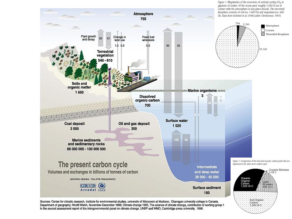
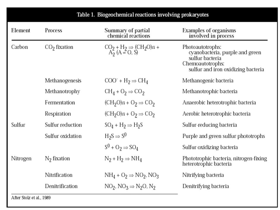
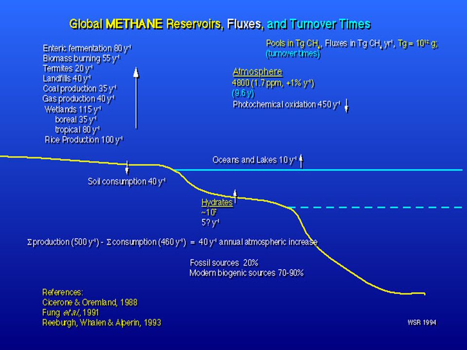
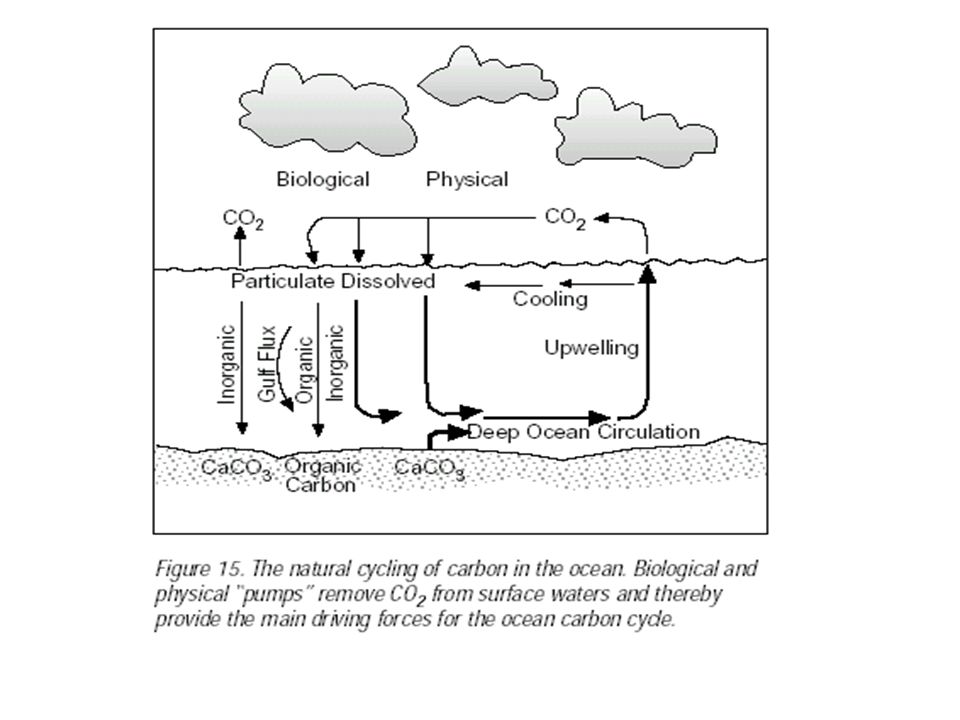
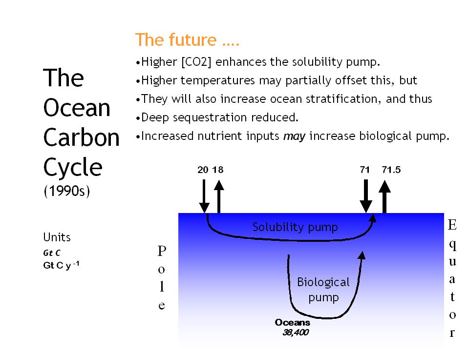
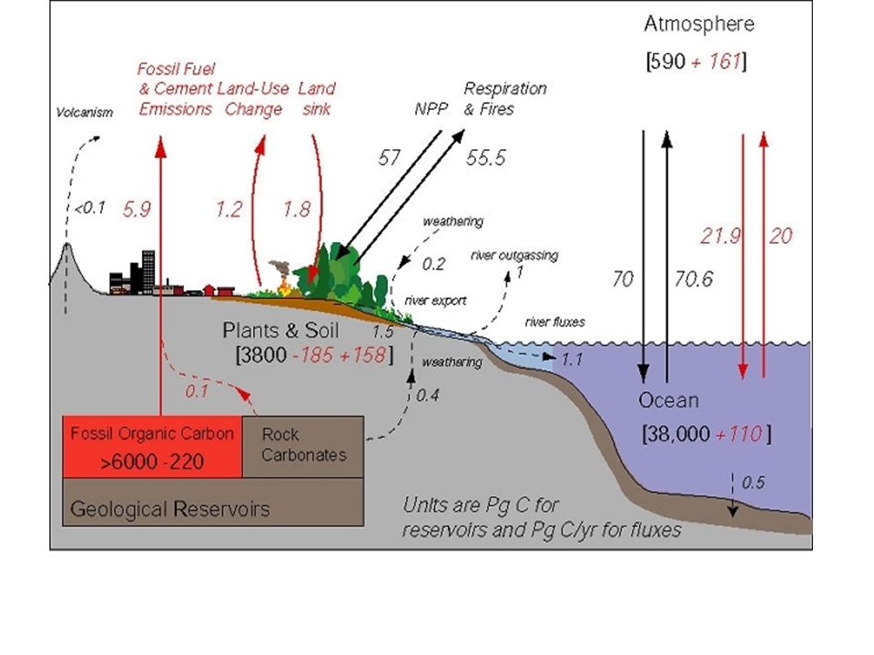
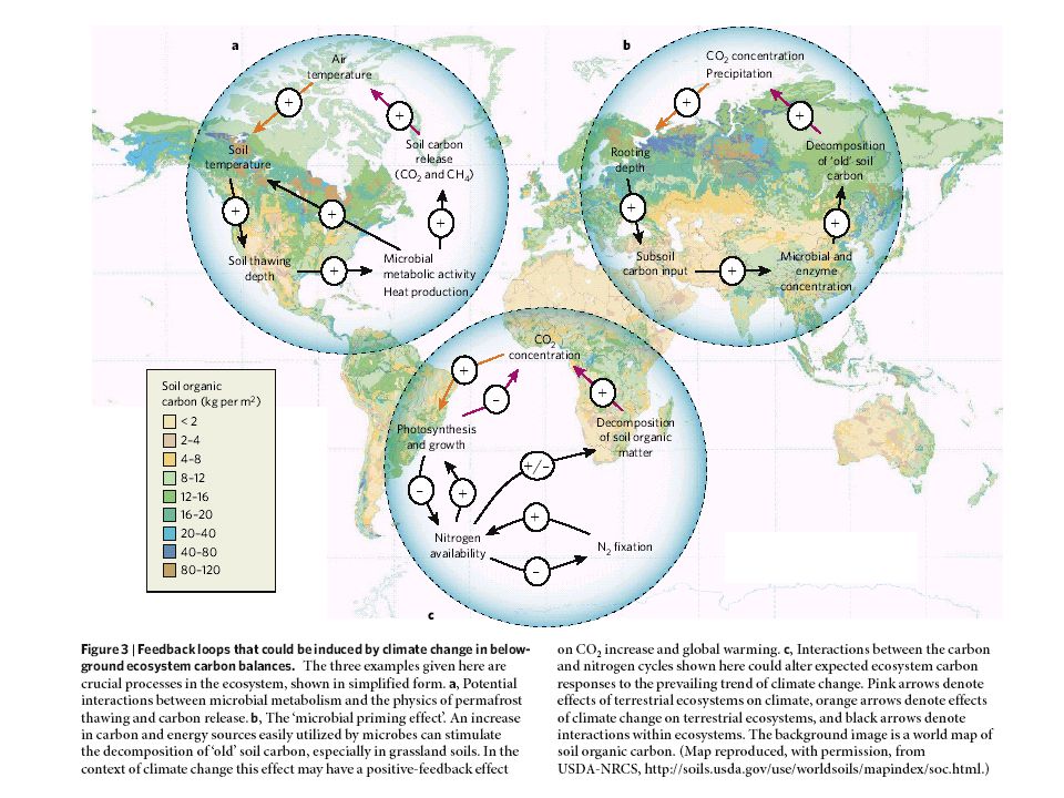
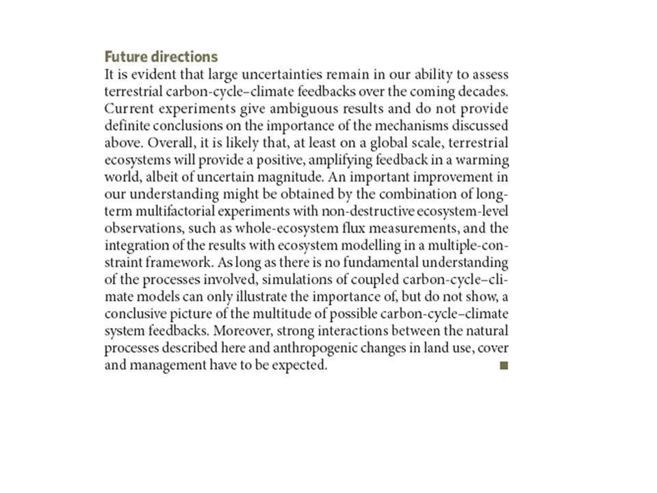
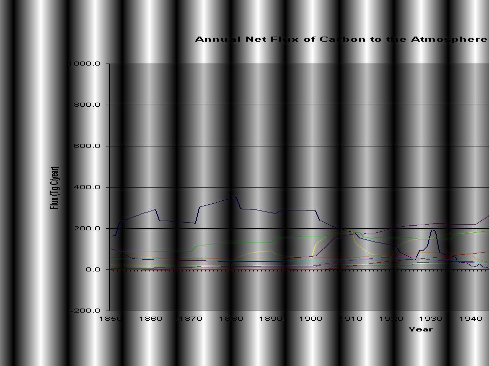
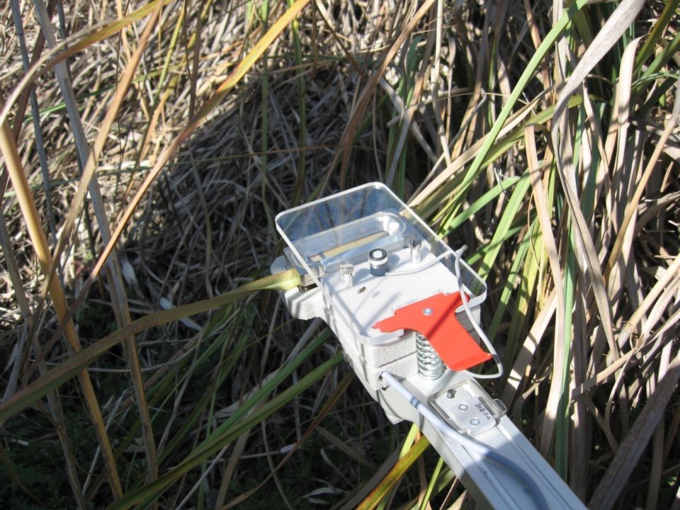
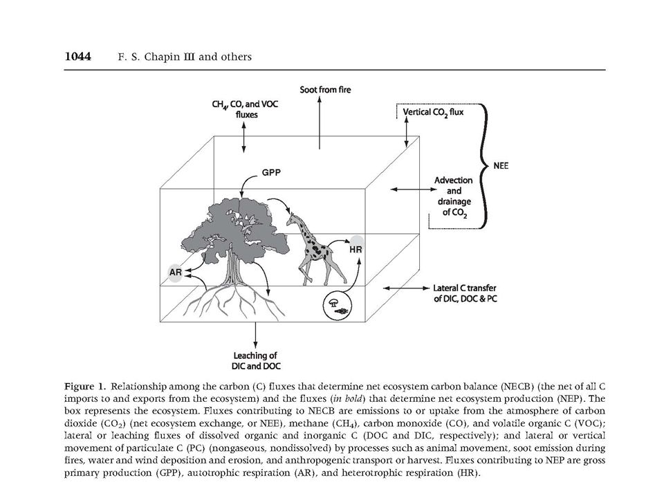
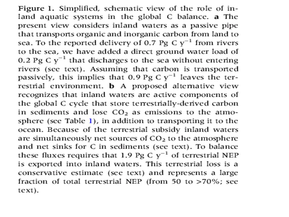
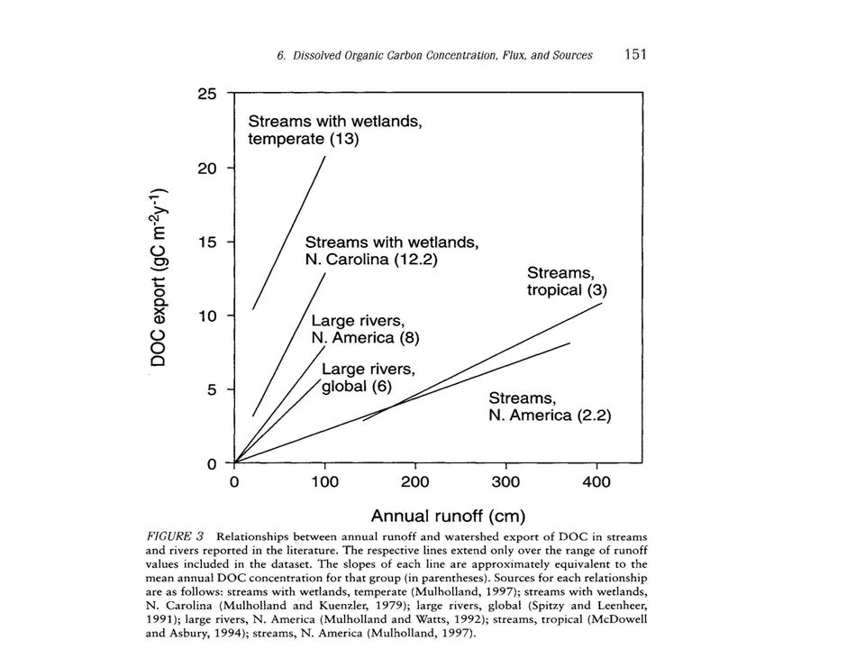
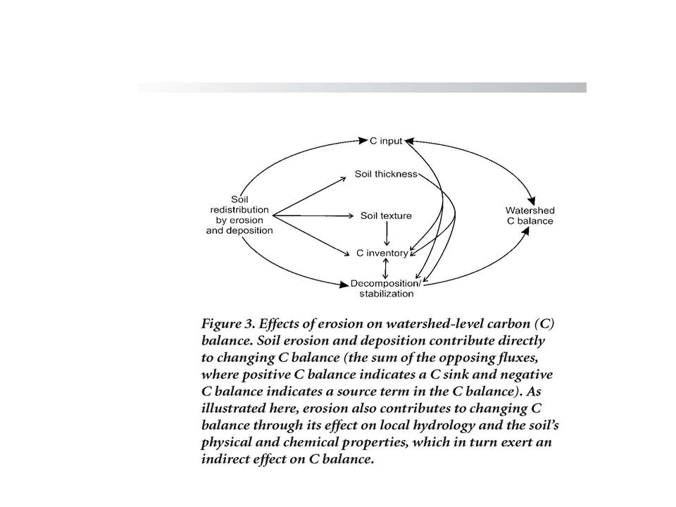
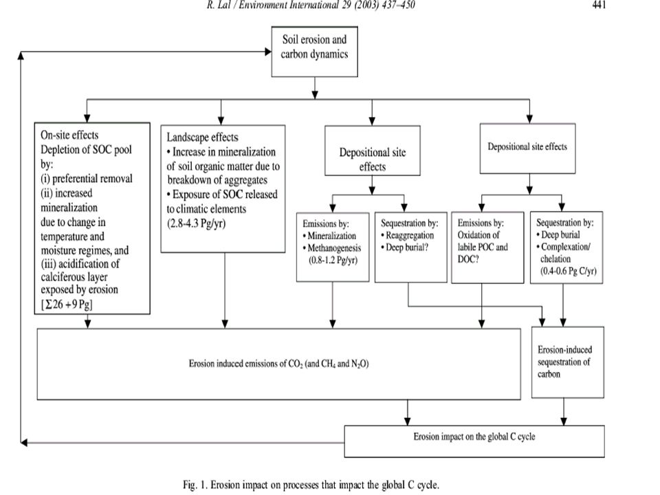
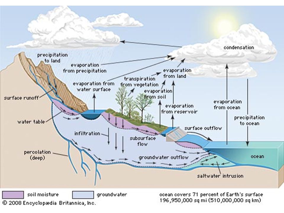
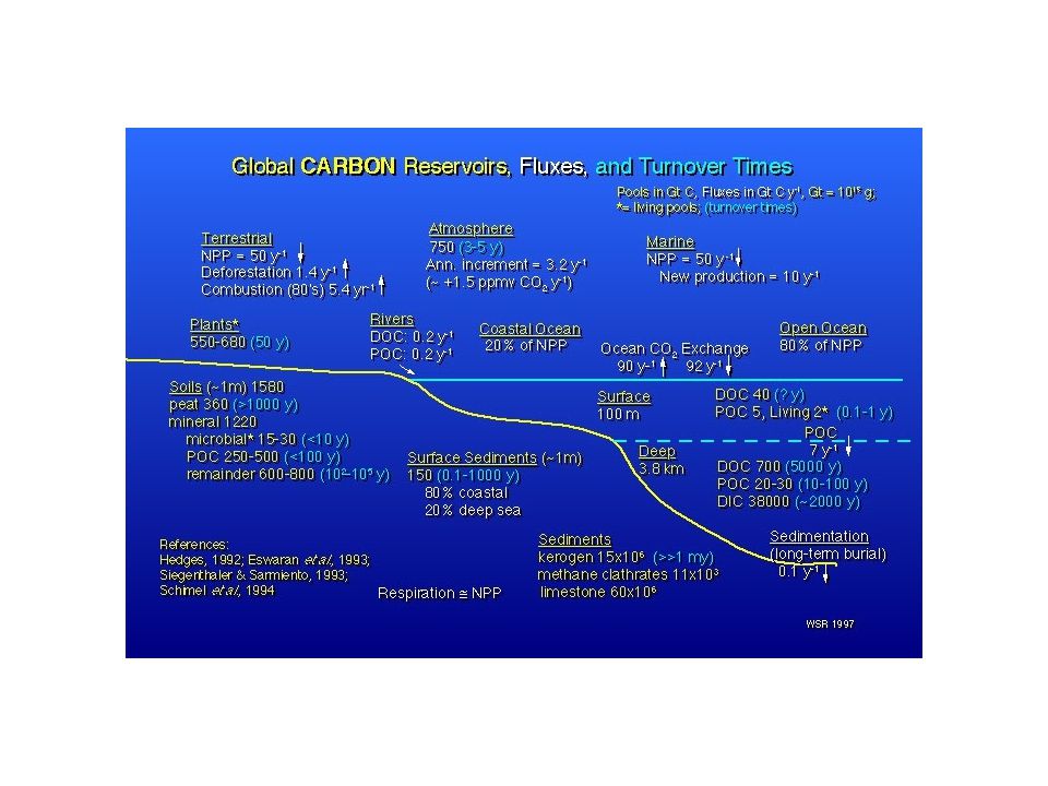
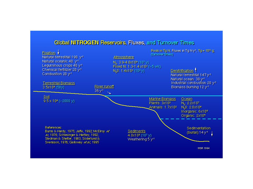
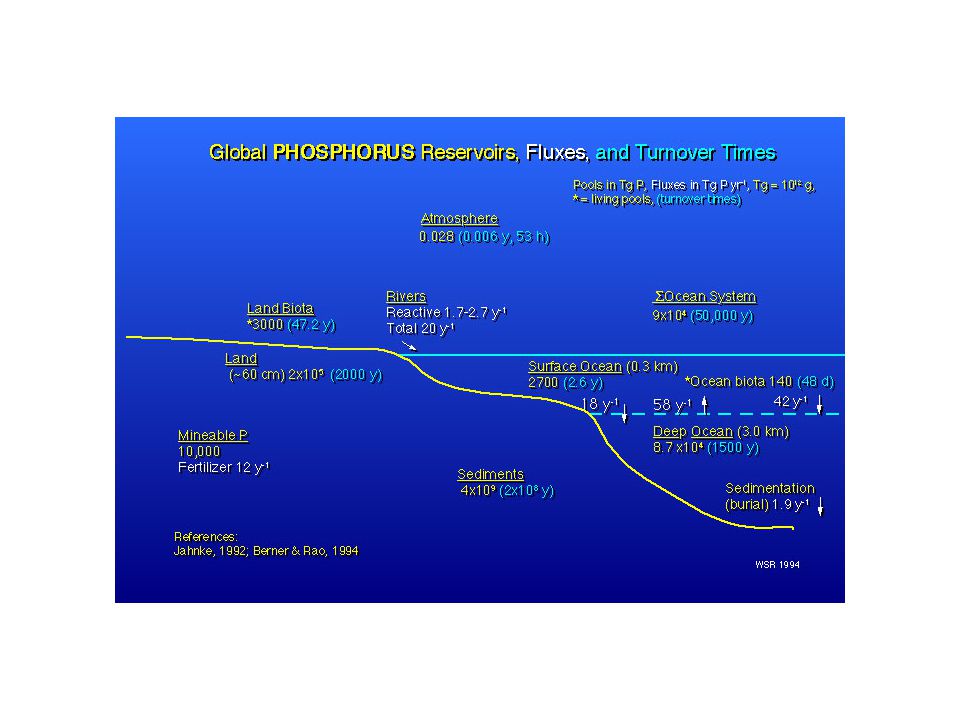
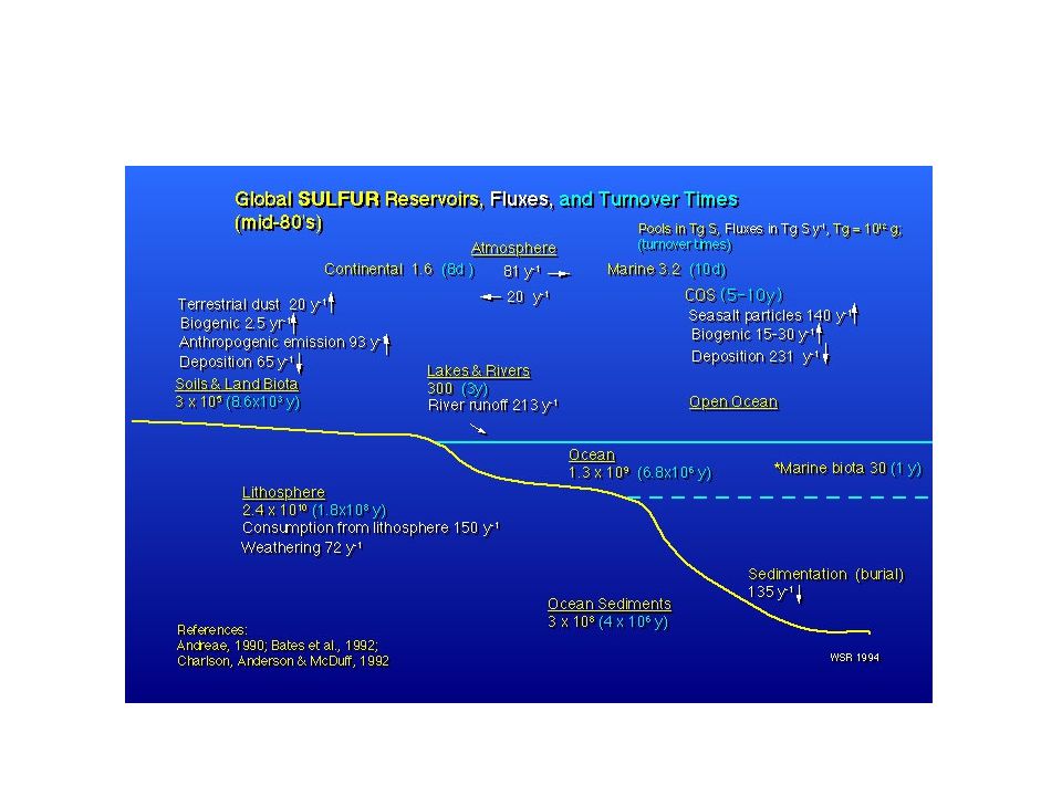
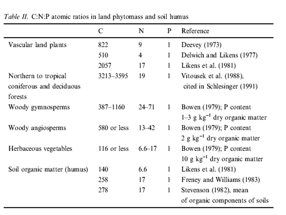
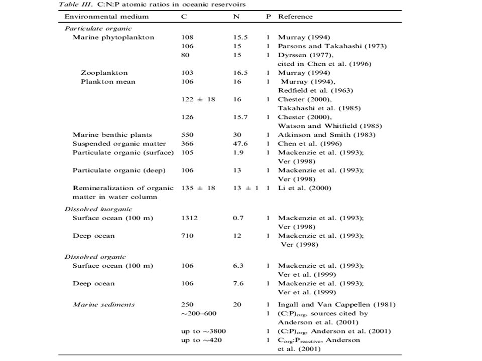


 Oxígeno Oxygen (O 2 ) 2 La Fotosíntesis de las plantas producen Oxígeno Photosynthesis of plants produces Oxygen.>")

—to melt rock. This.>")


