5º Máster “Cambio global”

Presentación del tema: "5º Máster “Cambio global”"— Transcripción de la presentación:

1 5º Máster “Cambio global”
(Palma de Mallorca, octubre de 2013) Módulo 2.02: “Impactos del Cambio Global sobre la hidrología y los ciclos biogeoquímicos en cuencas hidrográficas” Tema 15: “Ciclo global contemporáneo del carbono y cambios bajo un escenario de cambio climático” Juan Carlos Rodríguez Murillo, científico titular, Museo Nacional de Ciencias Naturales, CSIC

2 El ciclo global del carbono The global carbon cycle
Introducción /Introduction 2) Descripción general del ciclo del carbono / General description of carbon cycle 3) Depósitos del ciclo (rápido) del carbono / Reservoirs of the (fast) carbon cycle 4) Impactos del cambio global en el ciclo del carbono / Global change impacts on carbon cycle 5) Métodos de estimación de depósitos y flujos de carbono / Methods of estimation of reservoir and carbon fluxes

3 El carbono en la Tierra / Carbon on Earth
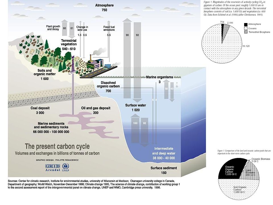
Introducción El carbono en la Tierra / Carbon on Earth Es el elemento clave de los seres vivos. / Carbon is the key element for living beings El ciclo del carbono incluye al carbono orgánico en todas sus formas (la totalidad de los seres vivos y de las moléculas orgánicas), así como al C inorgánico, fundamentalmente en forma de CO, CO2 y (bi) carbonatos. / Carbon cycle includes organic carbon in all forms (all the living beings and organic molecules), as well as inorganic carbon, mostly as CO, CO2 and (bi) carbonates Los flujos de carbono en el ciclo están asociados a procesos bioquímicos (fotosíntesis y respiración), físicoquímicos (disolución de CO2 en el agua), químicos (meteorización de silicatos, disolución y precipitación de carbonatos) y físicos (erosión, transporte y deposición). / Carbon fluxes are associated to biochemical (photosynthesis and respiration), physicochemical (CO2 dissolution in water), chemical (silicate weathering, carbonate dissolution and precipitation) and physical (erosion, transport, and deposition)

4 El carbono en la Tierra/ Carbon on Earth
El compuesto fundamental del ciclo del carbono es el dióxido de carbono (CO2)./ CO2 is the basic compound in the carbon cycle Este gas es prácticamente inerte en la atmósfera, pero soluble en el agua, y materia prima de la fotosíntesis y producto de la respiración./ CO2 is practically inert in the atmosphere, but is water soluble, and is the photosynthesis raw material, as well as a main product of respiration Por ello, el CO2 es el componente fundamental de los flujos de C entre la atmósfera y la biosfera y la atmósfera y los océanos. /Therefore, CO2 is the main compound in biosphere-atmosphere and ocean-atmosphere C fluxes Además, por su participación en la meteorización de los silicatos y en la disolución y precipitación de carbonatos, contribuye al reciclado de volátiles a través de la litosfera y forma las rocas sedimentarias carbonatadas. Aditionally, CO2 contributes to volatile recycling through lithosphere, and produces sedimentary limestones by its role in silicate weathering and carbonate dissolution and precipitation, respectively.

5 2) Descripción general del ciclo del carbono / General description of carbon cycle

6 El ciclo del C, como el de cualquier elemento o materia, puede considerarse constituído por depósitos y flujos. La variación temporal del contenido “C” de un depósito, será: dC/dt = (Flujo de entrada de C) – (Flujo de salida de C) En estado estacionario, ambos flujos son iguales, así que: dC/dt = 0, con lo que C es constante. El tiempo de residencia del C en cada depósito será = (Tamaño del depósito/flujo de salida). /Admitting steady-state, Cturnover in each reservoir is = (Reservoir size / Output flux)

7

8 Figure 1. Cartoon of fluxes (arrows) and inventories (number in boxes) of the labile components of the global carbon system for the 1980's. The red arrows are the perturbation fluxes resulting from emissions of anthropogenic CO2. From Sabine et al. (2003).

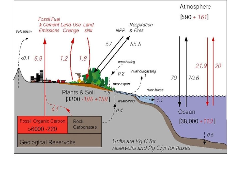
9 The schematic highlights carbon fluxes through inland waters5, and also includes pre-industrial2 and anthropogenic3 fluxes. Values are net fluxes between pools (black) or rates of change within pools (red); units are Pg C yr-1; negative signs indicate a sink from the atmosphere. Gross fluxes from the atmosphere to land and oceans, and the natural (Nat) and anthropogenic (Ant) components of net primary production — the net uptake of carbon by photosynthetic organisms — are shown for land and oceans. Gross primary production (GPP) and ecosystem respiration (R) are poorly constrained18, 19; we therefore modified respiration to close the carbon balance. Non-biological dissolution of anthropogenic carbon dioxide by the oceans is included in these fluxes2. Fluxes to the lithosphere represent deposition to stable sedimentary basins, and the flux from the lithosphere to land represents erosion of uplifted sedimentary rocks2. (Nature Geoscience 2, (2009) doi: /ngeo618 The boundless carbon cycle Tom J. Battin, Sebastiaan Luyssaert, Louis A. Kaplan, Anthony K. Aufdenkampe, Andreas Richter& Lars J. Tranvik )

10 El CO2 atmosférico es estable químicamente
El CO2 atmosférico es estable químicamente. Su vida media atmosférica es de 750 Gt/( Gt año-1) ó 3,5 años, antes de entrar en los ecosistemas terrestres o en los océanos. / Atmospheric CO2 is chemically stable, with an average atmospheric lifetime of 3.5 years, before entering terrestrial ecosystems or oceans. Flujos atmósfera-tierra: - Fotosíntesis (CO2 + H 2O CH2O + O2) - Respiración (oxidación) - Flujos geoquímicos (meteorización de silicatos, reacciones con carbonatos, metamorfismo) Flujos atmósfera-océano: - Disolución de CO2 (CO2 + H2O HCO3- + H+ HCO CO3-2 + H+ ) - Desgasificación de CO2

11 Ciclos del carbono “rápido” y “lento”/ “Slow” and “fast “ carbon cycles
Los depósitos geológicos de C (carbonatos de los sedimentos y C orgánico en forma de querógeno o combustibles fósiles) tienen tiempos de residencia de cientos de millones de años. / C turnover in geological reservoirs (sedimentary limestone and organic C as kerogen) takes hundreds of million years Los depósitos de C atmosférico, biosférico y oceánico superficial intercambian C en años o decenas de años. / Atmospheric, biospheric and shallow sea reservoirs have turnover times of years or tens of years El C tiene unos 500 años de tiempo de residencia en el depósito oceánico total. / Turnover of C in the whole ocean takes about 500 years

12 Podemos, pues, distinguir un ciclo lento geológico, de flujos lentos que determinan la concentración atmosférica del CO2 a escalas de millones de años, y un ciclo rápido biogeoquímico, que influye en dicha concentración a escala de decenios-centenas de años. /We may differentiate a geological slow cycle, made of slow fluxes which determine the atmospheric CO2 concentration in the million-year range, and a biogeochemical fast cycle, which establishes CO2 concentration in the short term (decade – centennial)

13 Otros procesos del ciclo del carbono / Other processes
in the carbon cycle - Procesos del ciclo geológico del carbono / Processes in carbon geological cycle 1) Meteorización de silicatos: CaSiO3 + 2CO2 + H2O Ca HCO3 +SiO2 2) Precipitación/disolución de carbonatos: Ca2+ + 2HCO CaCO3 + CO2 + H2O 3) Metamorfismo: CaCO3 + SiO CaSiO3 + CO2 - Procesos del subciclo del metano /Methane subcycle processes

14 El subciclo del metano / The methane subcycle
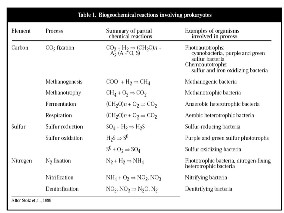
Dentro del ciclo del carbono, “movido” mayoritariamente por el CO2 , podemos distinguir un subciclo, cuyo componente dinámico es el metano (CH4). / As a part of C cycle, one can analyze a methane (CH4) subcycle El metano es la “parte anaerobia” del ciclo del carbono, ya que su producción requiere la ausencia de oxígeno./ Methane represents the “anaerobic side” of carbon cycle, because its production needs oxygen absence

15 Generación / descomposición de metano
La generación de metano se produce en el metabolismo de diferentes procariotas (bacterias metanogénicas) por descomposición del acetato (dando CO2 como subproducto) o por reducción del CO2 con H2 (reducción disimilatoria de CO2 )./ Methane generation occurs in methanogenic bacteria metabolism, by acetate decomposition (giving CO2 as byproduct) or by H2 mediated CO2 reduction (dissimilatory CO2 reduction) El consumo de metano se produce también por oxidación con O2 en bacterias (metanotróficas), por oxidación con sulfato (bacterias sulfato- reductoras), y por oxidación atmosférica con el radical hidroxilo./ Methane consumption occurs by O2 oxidation in bacteria (methanotrophic), by oxidation with sulfate (sulfate-reducing bacteria), and by atmospheric oxidation with hydroxyl radical.

16

17

18

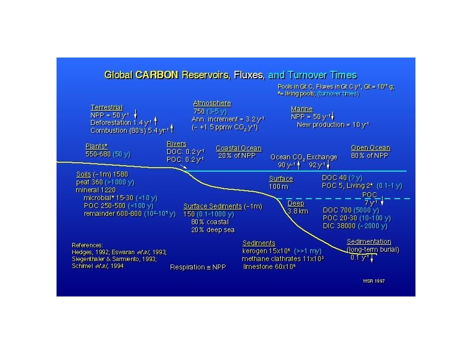
19 Atmosphere 3.2 63.0 750 6.3 1.6 Fossil Deposits 60 Plants 91.7 About 4,100 500 Soil 90 Units Gt C Gt C y -1 2000 0.7 Oceans 38,400 3) DEPÓSITOS DEL CICLO (RÁPIDO) DEL CARBONO /Reservoirs of the (fast) carbon cycle

20 LA ATMÓSFERA LA ATMÓSFERA

21 La atmósfera primitiva y la actual / Primeval and present atmosphere
Las masas de agua, C, N y S en la superficie terrestre actual son casi las mismas de las de los compuestos volátiles que constituían la atmósfera de la Tierra primitiva./ Masses of water, C, N, and S on the present Earth surface are almost equal to those of the volatile compounds which made up the primitive Earth atmosphere La atmósfera primitiva procedente de la desgasificación de estos compuestos volátiles contenía agua (90%) y CO2 (7-8%), con algo de N2 , HCl y H2S./ Primeval atmosphere from volatilization of these volatile compounds contained water (90%) and CO2 (7-8%), with minor quantities of N2 , HCl y H2S Al enfriarse la Tierra, el agua se condensó, disolviendo a todos los volátiles menos el N2. La atmósfera quedó formada por nitrógeno y CO2./ As Earth cooled, water condensed, dissolving volatiles except N2 . Only CO2 and N remained in the atmosphere La concentración atmosférica de CO2 en el Precámbrico fue disminuyendo por formación de carbonatos y de materia orgánica./ The CO2 atmospheric concentration in Precambric was falling by carbonate and organic matter formation

22 El CO2 a través de la historia geológica
Aumento de CO2 : Desgasificación (vulcanismo, tectónica). Disminución de CO2 : Meteorización, depósitos de materia orgánica).

23 El CO2 a través de la historia geológica: El Pleistoceno

24 El CO2 reciente

25 Atmospheric Concentration
The pre-industrial (1750) atmospheric concentration was 278ppm This has increased to 390ppm in 2011, a 40% increase “Seasonally corrected” is a moving average of seven adjacent seasonal cycles Source: NOAA/ESRL; Global Carbon Project 2012

26 El metano atmosférico reciente
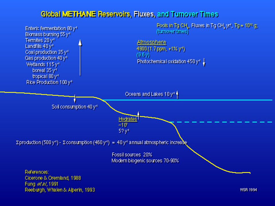
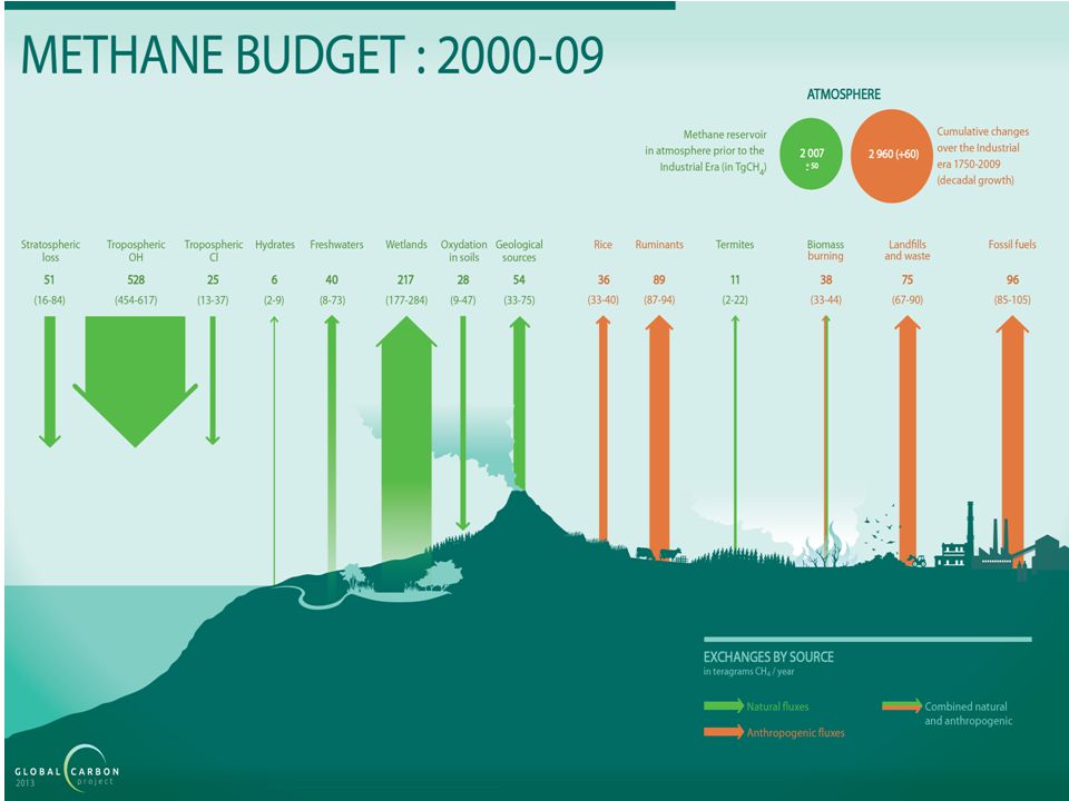
: 12 ± 6 ppb : 6 ± 8 ppb : 2 ± 2 ppb Aumento hasta el 2000 Prácticamente cte. hasta 2005 Aumenta hasta 2010 (últimos datos disponibles) No se conoce la razón de las variaciones de las concentraciones de metano en la atmósfera.

27 LOS OCÉANOS

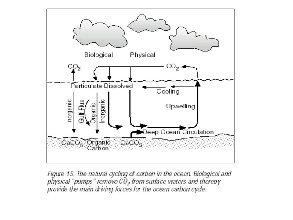
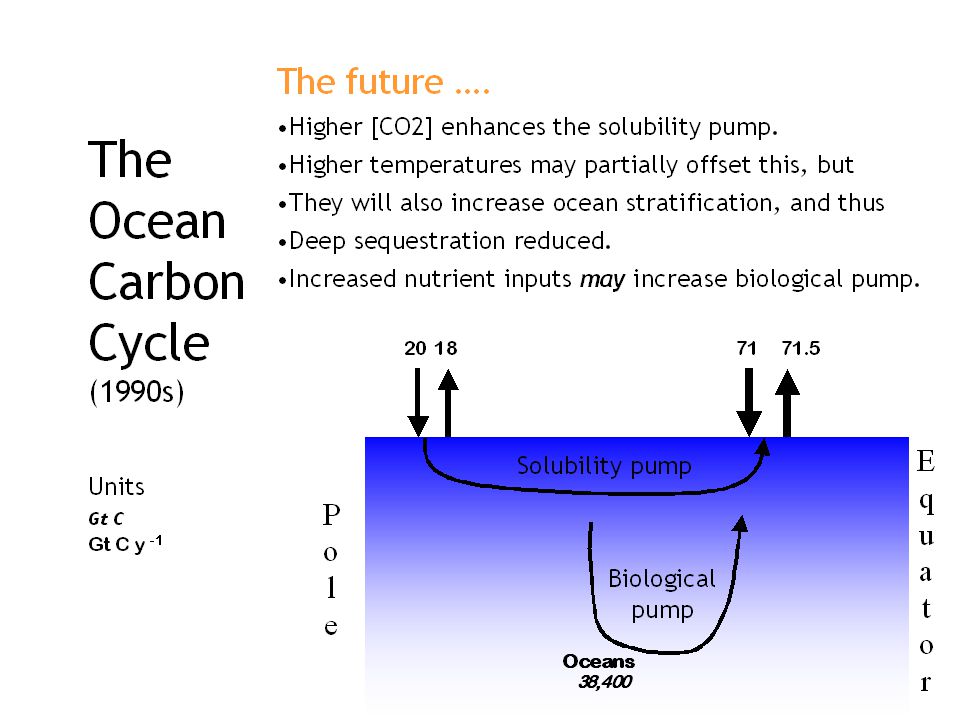
28 Los océanos : Cambios en el dióxido de carbono disuelto/
Oceans: Changes in dissolved carbon dioxide

29

30

31 LOS ECOSISTEMAS TERRESTRES

32 Global Carbon Stocks (Gt C)
Table 1: Global carbon stocks in vegetation and soil carbon pools down to a depth of 1 m. Biome Area (109 ha) Global Carbon Stocks (Gt C) Vegetation Soil Total Tropical forests 1.76 212 216 428 Temperate forests 1.04 59 100 159 Boreal forests 1.37 88 471 559 Tropical savannas 2.25 66 264 330 Temperate grasslands 1.25 9 295 304 Deserts and semideserts 4.55 8 191 199 Tundra 0.95 6 121 127 Wetlands 0.35 15 225 240 Croplands 1.60 3 128 131 15.12 466 2011 2477 Note: There is considerable uncertainty in the numbers given, because of ambiguity of definitions of biomes, but the table still provides an overview of the magnitude of carbon stocks in terrestrial systems.

33 Total C en vegetación: 466 Gt Total C en suelos: 2.011 Gt
(IPCC, 2000, “Land use, land-use change and forestry”)

34 Land-Use Change Emissions
Global land-use change emissions: 0.9±0.5PgC in 2011 The data suggests a general decrease in emissions since 1990 Peat fires Black line: Includes management-climate interactions; Thin line: Previous estimate Source: Le Quéré et al. 2012; Global Carbon Project 2012

35 4) Impactos del cambio global en el ciclo del carbono / Global change impacts on carbon cycle

36 Anthropogenic Perturbation of the Global Carbon Cycle
Perturbation of the global carbon cycle caused by anthropogenic activities, averaged globally for the decade 2002–2011 (PgC/yr) Source: Le Quéré et al. 2012; Global Carbon Project 2012

37

38 Changes in the Global Carbon Budget over Time
The sinks have continued to grow with increasing emissions It is uncertain how efficient the sinks will be in the future Source: Le Quéré et al. 2012; Global Carbon Project 2012

39 Global Carbon Budget Emissions to the atmosphere are balanced by the sinks Averaged sinks since 1959: 44% atmosphere, 28% land, 28% ocean The dashed land-use change line does not include management-climate interactions The land sink was a source in 1987 and 1998 (1997 visible as an emission) Source: Le Quéré et al. 2012; Global Carbon Project 2012

40 (Woods Hole Research Center)

41 Las variaciones de la tasa de crecimiento de la concentración atmosférica de CO2 están causadas principalmente por efectos terrestres, particularmente por los impactos de las olas de calor y las sequías en la vegetación de la Amazonía occidental y del sudeste asiático, que producen pérdidas de C en los ecosistemas debido a la menor productividad vegetal y/o incremento de la respiración. / Fluctuations of atmospheric CO2 concentration growth rate are mainly the result of terrestrial effects, particularly of heathwave and drought impacts on Western Amazonia and Southeastern Asia vegetation, which cause a loss of ecosystem carbon due to lower plant production and/or increased respiration

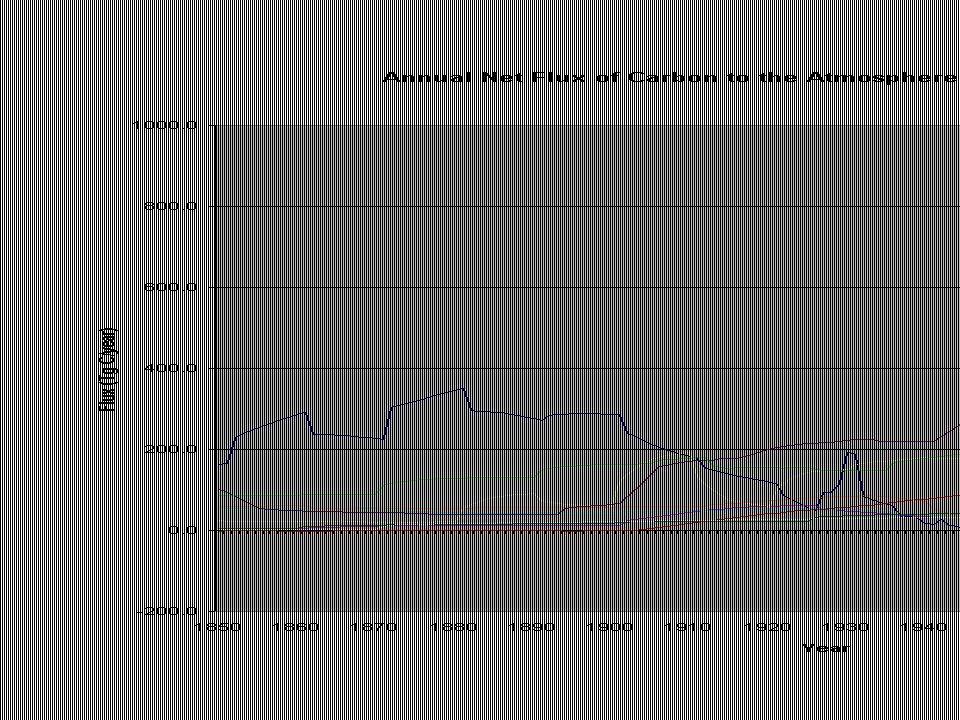
42 Inferred changes in CO2 flux compared with the 1980-98 mean Bousquet et al (2000) Science 290 1342
Land ̃ Oceans

43 Balance preindustrial de carbono: Casi en equilibrio (cambios lentos en el CO2 atm.)
Pequeña fuente en el océano. /Preindustrial C budget: Near equilibrium. Slow changes in atmospheric CO2. Small oceanic source Balance moderno de carbono: CF – A CF: Flujo por combustibles fósiles y cemento A: Aumento atmosférico de C Gran sumidero oceánico y sumidero variable en la biosfera. /Modern C budget: Big ocean sink and variable biospheric sink. Budget is = CF –A, CF being the C flux from fossil fuels and A the atmospheric C growth. Los flujos CF y A están muy bien caracterizados. La diferencia CF – A se ha de repartir entre la biosfera y el océano. Este reparto varía temporalmente y espacialmente. / CF and A fluxes are very well determined. CF –A must be shared between biosphere and ocean. Shares vary temporally and spatially. Los océanos absorben CO2 a altas latitudes (formación de aguas profundas –debido al downwelling- y lo emiten a bajas latitudes (por el upwelling) / Oceans absorb CO2 at high latitudes (by downwelling) and emit at low latitudes (by upwelling) El sumidero oceánico está bien relativamente bien caracterizado:/ Ocean sink is relatively well characterized Por los modelos de circulación oceánica./ By ocean circulation models Por las medidas de la evolución temporal del 13C./ By 13C temporal evolution measurements - Por las medidas de la evolución temporal del O2./ By O2 temporal evolution measurements

44 Balance mundial del carbono/
Global carbon budget 1980s 1990s Incremento atmosférico 3,3 ± ,1 ± 0.1 Emisiones “fósiles” 5,4 ± ,4 ± 0.4 Flujo océano - atmósfera -1,8 ± ,2 ± 0.4 Flujo tierra – atmósfera -0,3 ± 0,9 -1,1 ± 0,9 Flujo por cambios de uso 0,9 a 2,8 1,6 ± 0,7 Flujo residual terrestre -4,0 a -0, ,6 ± 0,9 El sumidero terrestre de carbono parecía intensificarse / The terrestrial carbon sink seemed to increase

45 Balance mundial del carbono/ Global carbon budget
( ) Incremento atmosférico 4,13 ± 0,1 Emisiones “fósiles” 7,7 ± 0,5 Flujo océano - atmósfera -2,3 ± 0,4 Flujo tierra – atmósfera -1,3 ± 1,0 Flujo por cambios de uso 1,1 ± 0,7 Flujo residual terrestre -2,4 ± 1,0 Se acelera la acumulación atmosférica de carbono / Atmospheric C accumulation increases Se intensifica el sumidero oceánico / Oceanic sink intensifies ¿Sumidero terrestre estabilizado?

46 Anthropogenic Global Carbon Dioxide Budget
Global Carbon Project 2010

47 El CO2 reciente y en un futuro cercano

48 ¿Cómo se comportarán los ecosistemas terrestres en el futuro?
Terrestrial ecosystem carbon dynamics and climate feedbacks Martin Heimann1 & Markus Reichstein 1 Nature 451, (17 January 2008) | Global terrestrial carbon uptake was simulated by 11 coupled carbon-cycle–climate models driven with carbon emissions from the SRES-A2 emissions profile. Data are taken from the Coupled Carbon Cycle Climate Model Intercomparison Project2, with uptake rates smoothed with a 30-year moving average.

49 ¿Dónde está el sumidero de C?

50

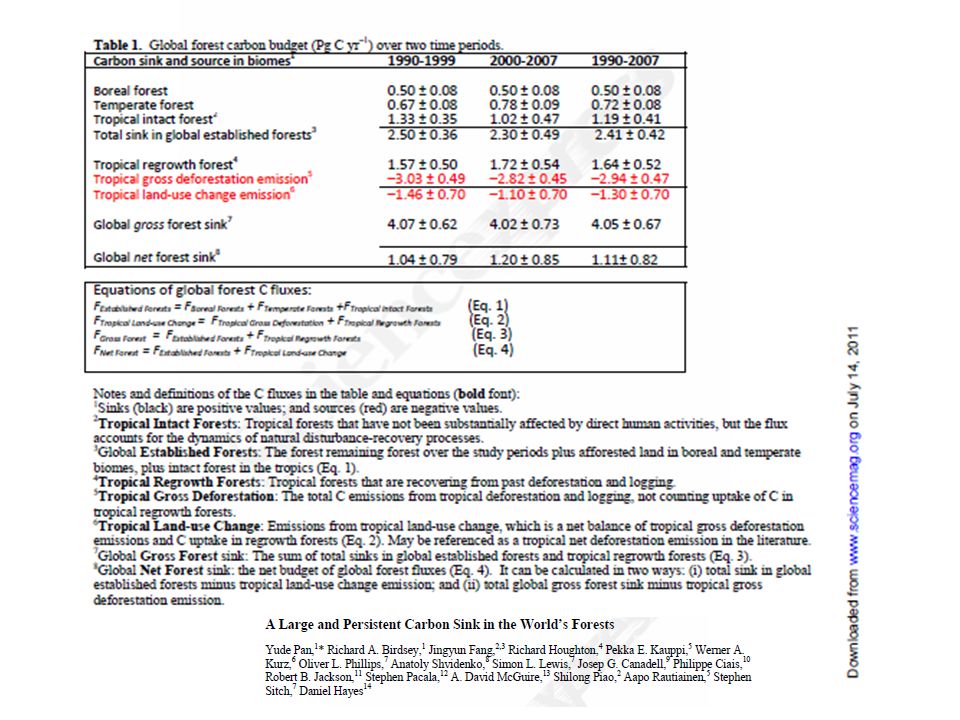
51 Los bosques son el tercer sumidero de C en la Tierra
(1,11 ± 0,82 Pg C/año, ) Los bosques dan cuenta de todo el flujo (neto) de C tierra-atmósfera Los bosques boreales y templados son sumideros netos (1,12 Pg C/año) Los bosques tropicales absorbieron 2,8 Pg C/año y emitieron 2,94 Pg/año (pequeña fuente neta)

52 Mecanismos propuestos para el sumidero terrestre de C/
Proposed mechanisms for terrestrial C sink Mecanismos fisiológicos: /Physiological mechanisms: Fertilización con CO2 / CO2 fertilization Fertilización con N / N fertilization Cambios de clima (T, humedad) / Climate changes (T, humidity) Mecanismos ecosistémicos:/ Ecosystemic mechanisms Recrecimiento forestal tras perturbaciones humanas./ Forest regrowth following human perturbation Menor deforestación./ Lower deforestation Supresión de incendios e “invasión” de matorrales./ Fire supression and bush encroachment Mejores prácticas agrícolas./ Better agricultural practices Productos forestales y vertederos./ Forest products and landfills Erosión y deposición de sedimentos./ Sediment erosion and deposition

53 El caso de los bosques Boreales: Cambios en la explotación, recrecimiento, más perturbaciones (fuego, plagas) Templados: Cambios en la explotación, recrecimiento, reforestación Tropicales: Deforestación, degradación, recrecimiento e incremento de biomasa en los bosques intactos.

54 Problemas para identificar y cuantificar los mecanismos de acumulación de carbono / Problems to identify and quantify carbon sequestration mechanisms Dificultad en determinar pequeñas variaciones de un gran sumidero (en especial, de los suelos)./ Difficulties to determine small changes in a big sink (specially soils) Dificultad en extrapolar los resultados de experiencias a pequeña escala hasta mayores escalas./ Difficulties to extrapolate small-scale experiences to bigger scales Deficiente representación en los modelos biosféricos de los procesos ecológicos relevantes para el ciclo del carbono./ Poor representation of carbon cycle relevant ecological processes in current biospherical models

55 ¿Qué factores son más importantes en determinar el sumidero terrestre de carbono
NO SE SABE Y el interés de saberlo no es sólo académico. Dependiendo de cual sea la importancia de cada mecanismo, el sumidero podría aumentar, disminuir o desaparecer o cambiar a fuente. Esto representaría una diferencia de hasta cientos de ppm de CO2 en la atmósfera durante este siglo, con las correspondientes consecuencias.../ For example, different mechanisms for the terrestrial carbon sink will produce very different future behaviors. If CO2 fertilization is largely responsible for the terrestrial sink, then the sink might be expected to increase as CO2 levels continue to rise in the future. However, if the terrestrial sink is being primary caused from the recovery of past land use (e.g., ~ year old abandonment of agriculture in the temperate latitudes), then it is likely that the sink will eventually stop and disappear altogether in a few decades (Foley & Ramankutty, 2003).

56 Algunas conclusiones

57 5) Métodos de estimación de depósitos y flujos de carbono/
Methods of estimation of carbon reservoirs and fluxes Modelado inverso de datos oceánicos/ Inverse modelling of ocean data Modelado inverso de datos atmosféricos/ Inverse modelling of atmospheric data Inventarios (Modelos de uso de la tierra e inventarios forestales)/ Inventories (Land use models and forest inventories) Medida directa de flujos de CO2 (eddy correlation, IRGA)/ Direct CO2 flux measurements Modelos de vegetación y suelos/ Vegetation and soil models Medidas satelitales/ Satellite measurements

58 Appendix 1. Methods of Estimating Terrestrial Carbon Fluxes
Here we review some of the methods used to determine the size and geographic locations of terrestrial carbon fluxes. This is just a cursory overview of the topic. In a recent paper, House et al. (2003) provides a more complete review of the various methods of estimating terrestrial carbon sources and sinks. Methods for estimating the size and geographic pattern of the terrestrial carbon sink first arose from the so-called “atmospheric inversion” technique of flux estimation. In an inversion method, terrestrial carbon fluxes are inferred by having to fulfill the requirement that the global carbon budget has to be balanced. Thus, knowing the fossilfuel and land use sources of carbon and the amount of carbon stored in the atmosphere, one can estimate the terrestrial and oceanic sources or sinks by difference. Further, the ocean and terrestrial fluxes can be partitioned by one of three methods: 1) simultaneous measurements of atmospheric CO2 and O2; 2) observations of atmospheric d13C; or 3) oceanic uptake as estimated by an ocean carbon cycle model. The inverse modeling approach has the advantage of being global in scale, and of implicitly accounting for all the processes influencing the global carbon cycle. However, it has the disadvantage of not being able to isolate the individual contributions of the various processes controlling the carbon cycle. Furthermore, while inversion methods are able to provide reasonably accurate estimates of global sources and sinks of carbon, and even sufficiently accurate estimates of the latitudinal north-south partitioning of the fluxes, they do not provide accurate longitudinal breakdown of the fluxes, and of different regional fluxes. While inversion methods are useful, they are not sufficient to understand the functioning of the terrestrial carbon budget. More direct methods of observing the terrestrial sources and sinks of carbon have been developed. One such observational approach measures terrestrial carbon fluxes at the atmospheric boundary layer in flux towers using the “eddy covariance” technique. This technique takes advantage of the fact that transport in the boundary layer is dominated by turbulent eddies, and uses turbulence theory and sophisticated instruments to measure vertical fluxes of carbon dioxide. While flux measurements are useful to obtain terrestrial fluxes at local scales, they continue to

59 be plagued by measurement errors when turbulence is low (such as at night times), and also have difficulty scaling up to regional levels and to decadal time scales. Another method of estimating carbon fluxes directly is by using inventory methods. These methods are normally limited to observations of changes in aboveground biomass in forested ecosystems; from changes in biomass, sources or sinks of carbon can be inferred. The method has the advantage of comprehensively including all processes that affect an ecosystem, but has the disadvantage of having limited consideration of belowground processes and non-forested ecosystems. Finally, various numerical models have been used to estimate terrestrial sources and sinks of carbon. These models include representations of the processes that are thought to affect terrestrial carbon fluxes. In particular, the models include controls such as atmospheric CO2 concentration, climate variability and change, atmospheric nitrogen deposition, and in a few cases anthropogenic land use and land cover change. The models have the advantage of being able to isolate the individual contributions of the various processes influencing the terrestrial carbon budget. However, the models are only as good as our understanding of the processes, and moreover, they only include the processes that are currently hypothesized to influence the carbon budget. In addition to all the above approaches to estimating present-day terrestrial carbon fluxes, many experimental approaches are in use to understand how terrestrial ecosystems might respond to changing atmospheric carbon dioxide concentrations and climate. In laboratories, greenhouses, and open top chambers, plants are grown in conditions of increased (or decreased) ambient CO2 concentrations to evaluate their response. This method has been further extended to the plot or stand scale scale in the Free Air CO2 Enrichment (FACE) experiments which aims to estimate the ecosystem level response to increased CO2. Furthermore, many soil warming experiments around the world attempt to measure the response of microbial respiration to increased soil temperatures.

60 Fuentes y sumideros de C por inversión (Ciais et al., 2000)

61 -Variación reciente de CO2 y oxígeno.
- Emisiones antrópicas de C y variación de δ13C.

62 Partición de sumideros
entre tierra y océanos por medidas del oxígeno. (Manning & Keeling) Tellus 58B (2006)

63 Figure 3.4: Partitioning of fossil fuel CO2 uptake using O2 measurements (Keeling and Shertz, 1992; Keeling et al., 1993; Battle et al., 1996, 2000; Bender et al., 1996; Keeling et al., 1996b; Manning, 2001). The graph shows the relationship between changes in CO2 (horizontal axis) and O2 (vertical axis). Observations of annual mean concentrations of O2, centred on January 1, are shown from the average of the Alert and La Jolla monitoring stations (Keeling et al., 1996b; Manning, 2001; solid circles) and from the average of the Cape Grim and Point Barrow monitoring stations (Battle et al., 2000; solid triangles). The records from the two laboratories, which use different reference standards, have been shifted to optimally match during the mutually overlapping period. The CO2 observations represent global averages compiled from the stations of the NOAA network (Conway et al., 1994) with the methods of Tans et al. (1989). The arrow labelled ?fossil fuel burning? denotes the effect of the combustion of fossil fuels (Marland et al., 2000; British Petroleum, 2000) based on the relatively well known O2:CO2 stoichiometric relation of the different fuel types (Keeling, 1988). Uptake by land and ocean is constrained by the known O2:CO2 stoichiometric ratio of these processes, defining the slopes of the respective arrows. A small correction is made for differential outgassing of O2 and N2 with the increased temperature of the ocean as estimated by Levitus et al. (2000).

64 1ppm de CO2 en la atmósfera corresponde a unas 2 Gt de CO2
Balance moderno de carbono: CF – A CF: Flujo por combustibles fósiles y cemento A: Aumento atmosférico de C Variación : CF= 30 ppm A=15 ppm 1ppm de CO2 en la atmósfera corresponde a unas 2 Gt de CO2 Variación O2 : 7 ppm ( ) Es decir, se han consumido 40 ppm de O2 en quemar los CF, pero en la atmósfera la disminución ha sido de 33 ppm. Por lo tanto, han aparecido 7 ppm de O2 en la atmósfera. Una molécula de CO2 que absorbe el océano no supone cambios en el O2 atmosférico. Una molécula de CO2 que se fija en la biosfera terrestre supone la emisión de una molécula de O2 . Por ello, las 7 ppm de O2 añadidas a la atmósfera, implican 7 ppm fijadas en la biosfera terrestre, y 15-7 = 8 ppm absorbidas por los océanos.

65 Métodos de inventario Modelos de uso de la tierra (Houghton, 1983)

66

67 Inventarios forestales
MODELO DEL CICLO DEL CARBONO FORESTAL (Rodríguez-Murillo, 1994)

68 Balance de carbono = Producción neta del bioma
FAC = (B + Rn + CE + CP)2 - (B + Rn + CE + CP)1 B (Biomasa viva): A partir de los VCC de los inventarios forestales. Rn (Residuos naturales): 0,1*B CE (Carbono edáfico): Su variación entre inventarios se considera proporcional a la variación de los VCC. CP (Depósitos provenientes de perturbaciones): Se estiman las entradas y salidas anuales a los 6 depósitos de carbono. Entradas: Estadísticas de incendios forestales, cortas, destino de la madera cortada y producción de leña. Salidas: Cada depósito se caracteriza por una tasa de oxidación constante R.

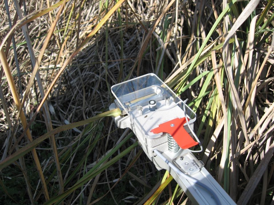
69 Torre con instrumentos para
medir los flujos netos de CO2 entre un ecosistema y la atmósfera (eddy correlation)

70 Medida del intercambio neto de CO2 en
hojas Medida de la respiración de suelos

71

72 Satélite japonés GOSAT (Ibuki) (Greenhouse
Gases Observing Satelite) ( ). Medida espectrométrica de CO2 , CH4 , vapor de agua y aerosoles Satélite estadounidense OCO (Orbiting carbon observatory). Lanzamiento fallido el Medida espectrométrica de CO2 Satélite europeo Envisat. Desde 2002. Observación de tierra, océanos, atmósfera y criosfera

73 Satélite Envisat. Observaciones de metano promediadas agosto-noviembre 2003

74 ©JAXA/NIES/MOEObservation period：August 1 –31, 2009
Satélite GOSAT. This figure shows a smoothed XCO2 distribution with mesh of latitude 2.5° x longitude 2.5°, calculated by applying statistical approach called Kringing method, which is essentially spatial inter- and extrapolation. Where observation points do not exist within 250km, the cell is shown as white.

75 GOSAT sigue funcionando.
Envisat dejó de estar operativo en marzo de 2012 OCO iba a ser lanzado de nuevo en febrero de 2013, pero la NASA ha suspendido la financiación por otro fallo del lanzador con otro satélite

76 5º Máster “Cambio global”
(Palma de Mallorca, octubre de 2013) Módulo 2.02: “Consecuencias hidrológicas y biogeoquímicas del Cambio Global en los ecosistemas continentales” Tema 16 “Conexiones entre los ciclos globales de agua, carbono, nitrógeno y fósforo” Juan Carlos Rodríguez Murillo, científico titular, Museo Nacional de Ciencias Naturales, CSIC

77 Conexiones entre los ciclos globales del agua, C, N y P/Interactions among global water, C, N, and P cycles

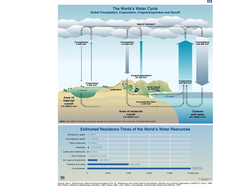
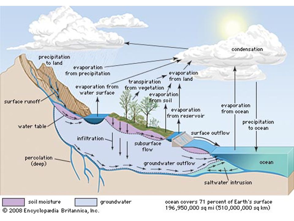
78 El ciclo hidrológico/Hydrologic cycle
El ciclo hidrológico constituye el vehículo de transporte directo de materia entre las tierras emergidas y los océanos. Por ello es importante en los ciclos biogeoquímicos básicos (C, O, N, P y S)./ Water cycle is the direct means of matter transport between land and ocean, hence it is important in the basic biogeochemical cycles (C, O, N, P and S) Los ríos comunican los ciclos terrestre y marítimo de estos elementos, llevando cada año unos km3 de agua ( Gt) al mar./ Rivers communicate terrestrial and marine cycles of these elements, by carrying to the ocean about 36,000 km3 ( Gt) of water yearly En la atmósfera, el vapor de agua es el principal gas de invernadero./Atmospheric water is the main greenhouse gas

79

80

81

82

83

84

85 El ciclo hidrológico y los principales ciclos elementales/Water cycle and main elemental cycles
Ciclo del C: El mayor depósito activo de C está en los océanos./The biggest active C reservoir is in the oceans Los procesos oceánicos (disolución de CO2 en agua, precipitación/disolución de carbonatos, fotosíntesis y respiración) regulan la concentración atmosférica de CO2 a medio plazo (cientos o miles de años)./ Oceanic processes (CO2 water solution, carbonate precipitation/ solution, photosynthesis and respiration) regulate medium term atmospheric CO2 concentration-hundreds to thousands of years- El flujo directo de C tierra-océano (a través de los ríos) es pequeño (del orden de 0,9 Gt C/año, o el 0,5% del total, unas 200 Gt de PPB) comparado con los flujos atmosféricos de C, pero importante en el balance terrestre del carbono./ Direct land-ocean C flux (through rivers) is small (about 0.9 Gt C/year, to be compared to about 200 Gt of GPP), but important in terrestrial carbon budget

86 El ciclo hidrológico y los principales ciclos elementales/Water cycle and main elemental cycles
Ciclo del N: Los óxidos de nitrógeno y las sales de N son muy solubles en agua. También acompaña N orgánico (aprox. el 10%) al C que fluye a los mares. Por ello, el flujo tierra-océano de N es mucho más importante en el ciclo del N que en el del C (60 Mt N/año, o una quinta parte de los flujos hacia la atmósfera –casi 300Mt/año-). Ciclo del P: Al carecer prácticamente el P de especies gaseosas en su ciclo terrestre, la inmensa mayoría del transporte de este elemento (>95%; 21 Mt/año de P) se hace vía ríos. Ciclo del S: Al tener los compuestos de S una vida atmosférica muy corta (horas-días), la principal vía de transporte entre tierra y mar son los ríos (130 Mt/año de S). Este flujo es casi la mitad del flujo total atmosférico de S (unos Mt/año).

87 En resumen: Cycle C N S P Water 900 60 130 21 36*106 0,5 17 33 >95
Land-ocean flux (Mton yr-1) (rivers) 900 60 130 21 36*106 % Total land-ocean/atmosphere flux 0,5 17 33 >95

88 CONEXIONES ENTRE LOS CICLOS DE C, N Y P/ C,N and P cycles interactions
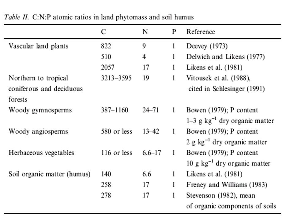
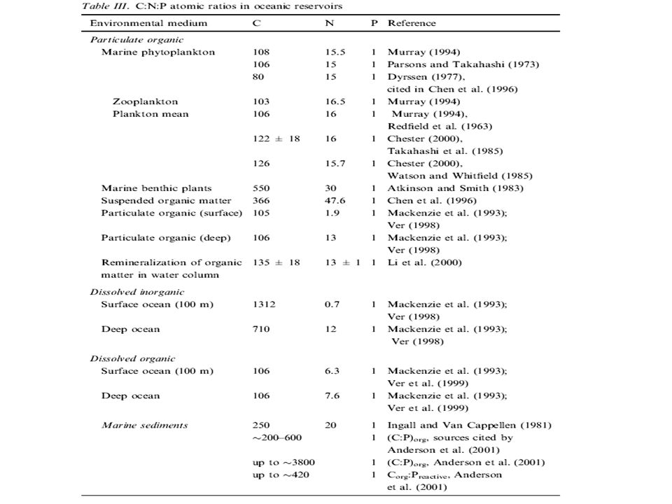
Los tejidos vivos se componen básicamente de C, O e H, pero más de 20 elementos adicionales son necesarios para la vida. Entre ellos destacan los llamados macronutrientes, al requerirse en grandes cantidades: N, P,S, K, Ca y Mg./ Live tissues are basically made of C, O, and H, but more than 20 additional elements are essential to live. In particular, big quantities of N, P,S, K, Ca, and Mg are required, and these elements are called macronutrients N, P y S son componentes fundamentales de las proteínas y otras biomoléculas (como los ácidos nucleicos), y son necesarios para el crecimiento vegetal. Al necesitarse en unas proporciones determinadas (aunque el valor depende del organismo), la fijación de carbono va acompañada también de la fijación de estos elementos en la materia viva./ N, P, and S are fundamental components of proteins and nucleic acids, and necessary to plant growth. Carbon fixation should be accompanied by the fixation of these elements in definite proportions

89 Element Symbol mg/kg percent Relative number of atoms Nitrogen N 15,000 1.5 1,000,000 Potassium K 10,000 1.0 250,000 Calcium Ca 5,000 0.5 125,000 Magnesium Mg 2,000 0.2 80,000 Phosphorus P 60,000 Sulfur S 1,000 0.1 30,000 Chlorine Cl 100 -- 3,000 Iron Fe Boron B 20 Manganese Mn 50 Zinc Zn 300 Copper Cu 6 Molybdenum Mo 1 Nickel Ni

90

91

92 El cambio global antropogénico en los ciclos de C, N, P y S
“Owing to land use activities and fossil fuel combustion, the terrestrial respiration and decay flux of CO2 to the atmosphere have increased by about 15%; the nitrogen fixation flux has more than doubled over its preindustrial rate; the mining of phosphate ores has led to emissions of four times more phosphorus to the surface environment than released by chemical weathering; and fossil fuel and biomass burning emissions have led to a doubling of the flux of sulfur to the atmosphere”. (Mackenzie, Ver y Lerman (2002) Chem. Geol 190, 13-32)

93 Fertilización con CO2 Las plantas C3 responden al aumento del CO2 con una mayor tasa fotosintética y un crecimiento mayor (mayor PPN). Esto no implica automáticamente un mayor almacenamiento de C en los ecosistemas, debido a: Aclimatación a las concentraciones mayores de CO2. 2) La disponibilidad de agua podría limitar el efecto del CO2 . 3) El almacenamiento es el resultado de muchos procesos. Se ha observado que el aumento de la PPN no suele reflejarse en aumentos del almacenamiento de C.

94 Fertilización con N (P)
Se cree que los ecosistemas templados están limitados en su PPN por el nitrógeno. Por lo tanto, el incremento de N debería aumentar la PPN. Si se mantienen las relaciones estequiométricas C:N, la adición de N debería producir una acumulación paralela de C en la biomasa y suelos. Sin embargo, el N podría inmovilizarse o perderse. Además, la adición de N viene en muchas ocasiones acompañada de acidificación, con los efectos negativos consiguientes sobre la productividad. No están claros los efectos a largo plazo del aumento en los nutrientes sobre los ecosistemas terrestres.

95

96