Descargar la presentación
La descarga está en progreso. Por favor, espere

1
Precipitación orográfica en climas fríos y cálidos
Cascadas (Oregon) Alpes Himalayas Esta presentacion es parte de un estudio que hemos desarrollado en el grupo donde trabajo para tratar de entender como la topografia afecta a la precipitacion. Para estudiar el problema sobre climas frios, nos enfocamos sobre los Alpes (cerca de la frontera entre Italia y Suiza) y en la montanias Cascades (en el estado Oregon en Estados Unidos), ya que en estos lugares se llevaron a cabo experimentos de campo que nos dieron acceso a observaciones muy detallas. Para investigar el efecto sobre climas calidos, nos enfocamos en el area de los Himalayas al sur de Asia, que es una region de conveccion freuente y profunda que ocurren en presencia de topografia extrema. Estamos analizando otras areas pero hoy solo voy a presentar resultado de estas 3 regiones Altura (m) sobre el nivel del mar Socorro Medina Departamento de Ciencias Atmosféricas, Universidad de Washington, Seattle, EU Colaboradores: Anil Kumar , Robert Houze, Dev Niyogi y Ulirke Romatschke Centro de Ciencias de la Atmósfera, UNAM, México DF, 19 marzo 2009 1
 Alpes. Himalayas. Esta presentacion es parte de un estudio que hemos desarrollado en el grupo donde trabajo para tratar de entender como la topografia afecta a la precipitacion. Para estudiar el problema sobre climas frios, nos enfocamos sobre los Alpes (cerca de la frontera entre Italia y Suiza) y en la montanias Cascades (en el estado Oregon en Estados Unidos), ya que en estos lugares se llevaron a cabo experimentos de campo que nos dieron acceso a observaciones muy detallas. Para investigar el efecto sobre climas calidos, nos enfocamos en el area de los Himalayas al sur de Asia, que es una region de conveccion freuente y profunda que ocurren en presencia de topografia extrema. Estamos analizando otras areas pero hoy solo voy a presentar resultado de estas 3 regiones. Altura (m) sobre el nivel del mar. Socorro Medina. Departamento de Ciencias Atmosféricas, Universidad de Washington, Seattle, EU. Colaboradores: Anil Kumar , Robert Houze, Dev Niyogi y Ulirke Romatschke. Centro de Ciencias de la Atmósfera, UNAM, México DF, 19 marzo")
2
Sponsored in part by: NSF Award# ATM NSF Award# ATM NASA Award# NNX07AD59G

3
Áreas de estudio para climas fríos
Suiza Italia

4
Precipitación climatológica (sep a nov) y contorno topográfico = 800 m
La climatologica de precipitacion durante las temporadas mas lluviosas en ambas regiones indica el efecto profundo que tiene la topografia en la distribucion de precipitacion. El flujo del viento en niveles altos (500 mb) durante las estaciones mostradas tienen a ser en la direccion de la flecha. Los sistemas meteorologico que dominan en estos lugares son ciclones extratropicales De manera que la ladera sur de los Alpes es la que normalemente esta a barlovento y por lo tanto tiene a recibir el flujo humedo del Mediterraneo y las acumulaciones mas grandes de precipitacion, en particular en la region denominada Monte Lema
 durante las estaciones mostradas tienen a ser en la direccion de la flecha. Los sistemas meteorologico que dominan en estos lugares son ciclones extratropicales. De manera que la ladera sur de los Alpes es la que normalemente esta a barlovento y por lo tanto tiene a recibir el flujo humedo del Mediterraneo y las acumulaciones mas grandes de precipitacion, en particular en la region denominada Monte Lema.")
5
Precipitación climatológica (de dic a feb) y topografía
La climatologica de precipitacion durante las temporadas mas lluviosas en ambas regiones indica el efecto profundo que tiene la topografia en la distribucion de precipitacion. El flujo del viento en niveles altos (500 mb) durante las estaciones mostradas tienen a ser en la direccion de las flechas. Los sistemas meteorologico que dominan en estos lugares son ciclones extratropicales De manera que la ladera oeste de las Cascadas es la que esta a barlovento y por lo tanto recibe el flujo humedo del Pacifico y acumulaciones grandes de precipitacion como resultado del forzamineto topografico. Este tipo de distribucion donde la acumulacion de precipitacion es mayor en barlovento que a sotavento se observa no solamente en la climatologia sino en cada estacion y en los eventos individuales de precipitacion. Entonces el objetivo de esta parte del estudio era entender los mecanismos dinamicos y microfisicos que contribuyen a esta distribucion.
 durante las estaciones mostradas tienen a ser en la direccion de las flechas. Los sistemas meteorologico que dominan en estos lugares son ciclones extratropicales. De manera que la ladera oeste de las Cascadas es la que esta a barlovento y por lo tanto recibe el flujo humedo del Pacifico y acumulaciones grandes de precipitacion como resultado del forzamineto topografico. Este tipo de distribucion donde la acumulacion de precipitacion es mayor en barlovento que a sotavento se observa no solamente en la climatologia sino en cada estacion y en los eventos individuales de precipitacion. Entonces el objetivo de esta parte del estudio era entender los mecanismos dinamicos y microfisicos que contribuyen a esta distribucion.")
6
Objetivos (parte sobre climas fríos): 1
Objetivos (parte sobre climas fríos): 1. Investigar los procesos microfísicos de formación de precipitación en la ladera a barlovento Documentar como el flujo del aire asociado con un ciclón extra tropical es afectado por el terreno 1. So when a mid-latitude system moves over a mountain range, the precipitation over the windward slope is enhanced. 2. The first objective is to understand the microphysical processes of precipitation formation on the windward slopes. That is, the pathways thru which vapor is converted into precipitation. 3. These processes depend on how the airflow within the mid-latitude cyclone interacts with the terrain, so my second objective is to document this interaction.
: 1. Investigar los procesos microfísicos de formación de precipitación en la ladera a barlovento 2. Documentar como el flujo del aire asociado con un ciclón extra tropical es afectado por el terreno. 1. So when a mid-latitude system moves over a mountain range, the precipitation over the windward slope is enhanced. 2. The first objective is to understand the microphysical processes of precipitation formation on the windward slopes. That is, the pathways thru which vapor is converted into precipitation. 3. These processes depend on how the airflow within the mid-latitude cyclone interacts with the terrain, so my second objective is to document this interaction.")
7
Instrumentación de los experimentos
IMPROVE II = Improvement of Microphysical parameterization Altura media de la cresta = 2 km MAP = Mesoscale Alpine Program Altura media de la cresta = 3 km NOAA WP-3D La ventaja para este estudio es que contamos con el mismo tipo de instrumentacion y implementacion en los dos experimentos entonces obtuvimos bases de datos paralelas. S-Pol = Radar de doble polarización (banda S) VP = Radar de haz vertical = Sondeo
 VP = Radar de haz vertical. = Sondeo.")
8
Se analizaron las características de los casos que produjeron las acumulaciones de precipitación mas grandes 1. Condiciones sinópticas 2. Modificación del flujo del aire por el terreno 3. Estabilidad estática 4. Reflectividad e hidrometeoros

9
Se analizaron las características de los casos que produjeron las acumulaciones de precipitación mas grandes 1. Condiciones sinópticas 2. Modificación del flujo del aire por el terreno 3. Estabilidad estática 4. Reflectividad e hidrometeoros

10
Pronostico del ECMWF (12 h)
Ejemplo de caso en los Alpes UTC 20 Sep 1999 Atura geopotencial y temperatura a 500 mb 1. All of the storms that I’ll be describing occurred ahead of baroclinic troughs. 2.Here, I’m showing the 500 mb geopotential height field during the 1st Alpine event of interest, called IOP2b. 3.We see a trough approaching the Alps and the region of interest, indicated by the black square. Pronostico del ECMWF (12 h)
")
11
Ejemplo de caso en las Cascadas - 0000 UTC 14 Dic 2001
Altura geopotencial, vientos y temperatura a 500 mb 1.For the IMPROVE-2 cases, the 500 mb geopotential height also consisted of a trough approaching the experimental region (indicated by the black square). Pronostico del MM5(12 h)
. Pronostico del MM5(12 h)")
12
Condiciones sinópticas de los eventos de interés: ◘ Sistema baroclínico aproximándose a la barrera orográfica ◘ La dirección del viento conforme se acerca el sistema es prácticamente perpendicular al terreno 1.I’m not going to show the synoptic flow of the rest of the storms but they all occurred as a baroclinic system approached the respective orographic barrier and 2. They had upstream flow ~ 850 mb was nearly perpendicular to the terrain. This point is important because it indicates potential for orographic precipitation. 3.Next I will document the terrain-modified airflow

13
1. Condiciones sinópticas 2
1. Condiciones sinópticas 2. Modificación del flujo del aire por el terreno 3. Estabilidad estática 4. Reflectividad e hidrometeoros

14
Dirección de los cortes verticales
Sistemas intensos en los Alpes donde se recolectaron observaciones continuas (IOP, Intensive Observing Periods) Dirección de los cortes verticales 1.The methodology used consisted on constructing mean radar fields during periods of heavy precipitation. 2. I’ll be showing vertical cross-sections extending from the S-Pol radar to the Alps in NW to N directions depending on the prevailing direction of the low-level flow (1.5 km – 2.0 km) in each storm.
 Dirección de. los cortes. verticales. 1.The methodology used consisted on constructing mean radar fields during periods of heavy precipitation. 2. I’ll be showing vertical cross-sections extending from the S-Pol radar to the Alps in NW to N directions depending on the prevailing direction of the low-level flow (1.5 km – 2.0 km) in each storm.")
15
Velocidad radial (promedio de 3 h)
MAP IOP2b Velocidad radial (promedio de 3 h) m s-1 Tipo A 1.This figure shows a vertical cross section of mean radial velocity during MAP IOP2b 2.It extends from the S-Pol radar toward higher elevations. 3.The values are positive everywhere denoting flow away from the radar, that is from the valley toward the high terrain. 4.Over the valley there is a low-level jet that is rising over the first peak of the terrain. 5.Since this airflow pattern repeated in other storms and to distinguish it form a different scenario that I’ll show later on I will call this pattern Type A. (Time period: UTC 20 Sep 1999) NNW RADAR
 m s-1. Tipo A. 1.This figure shows a vertical cross section of mean radial velocity during MAP IOP2b. 2.It extends from the S-Pol radar toward higher elevations. 3.The values are positive everywhere denoting flow away from the radar, that is from the valley toward the high terrain. 4.Over the valley there is a low-level jet that is rising over the first peak of the terrain. 5.Since this airflow pattern repeated in other storms and to distinguish it form a different scenario that I’ll show later on I will call this pattern Type A. (Time period: UTC 20 Sep 1999) NNW. RADAR.")
16
Velocidad radial (promedio de 3 h)
MAP IOP3 Velocidad radial (promedio de 3 h) m s-1 Tipo A 1.Mean radial velocity for following MAP case (IOP3) also shows a low-level jet rising over the terrain, therefore it is also classified as a Type A storm. (Time period: UTC 26 Sep 1999) NNW RADAR
 m s-1. Tipo A. 1.Mean radial velocity for following MAP case (IOP3) also shows a low-level jet rising over the terrain, therefore it is also classified as a Type A storm. (Time period: UTC 26 Sep 1999) NNW. RADAR.")
17
Velocidad radial (promedio de 3 h)
MAP IOP5 Velocidad radial (promedio de 3 h) m s-1 Tipo A 1.Type A flow was also observed in MAP IOP5 case. (Time period: UTC 3 Oct 1999) N RADAR
 m s-1. Tipo A. 1.Type A flow was also observed in MAP IOP5 case. (Time period: UTC 3 Oct 1999) N. RADAR.")
18
Velocidad radial (promedio de 3 h)
MAP IOP8 Velocidad radial (promedio de 3 h) m s-1 Tipo B 1.The mean radial velocity in another MAP case (IOP8) shows a distinctly different structure: 2.In this case we see some negative values (in green) at low-levels (below 1 km) which indicate flow toward the radar, so the low-level flow is clearly not rising over the mountain. 3.The flow at higher levels (~2 km) is strong and cross-barrier. 4.There is a shear layer between the low-level air and the jet above. 5.Flows characterized by a shear layer will be called Type B. (Time period: UTC 21 Oct 1999) NW RADAR
 m s-1. Tipo B. 1.The mean radial velocity in another MAP case (IOP8) shows a distinctly different structure: 2.In this case we see some negative values (in green) at low-levels (below 1 km) which indicate flow toward the radar, so the low-level flow is clearly not rising over the mountain. 3.The flow at higher levels (~2 km) is strong and cross-barrier. 4.There is a shear layer between the low-level air and the jet above. 5.Flows characterized by a shear layer will be called Type B. (Time period: UTC 21 Oct 1999) NW. RADAR.")
19
Tipo B MAP IOP8 – Datos de radar en el avión P3
Viento en la dirección del corte vertical m s-1 Tipo B This is a cross-section of P-3 airborne radar analysis for the same storm and in the same cross-section as before. The wind velocity in the direction parallel to the cross-section shows that the shear layer extended over the windward slopes and that it rose over the terrain. (Time period: UTC 21 Oct 1999) NW SE
 NW. SE.")
20
Dirección de los cortes verticales
Sistemas intensos en las montañas Cascadas donde se recolectaron observaciones continuas Dirección de los cortes verticales 1. For the IMPORVE-2 cases I’ll show vertical cross-sections extending from the S-Pol radar to the east. I’ll also show P3 airborne radar analysis in a cross-section located ~40 km to the north.

21
Velocidad radial (promedio de 3 h)
IMPROVE-2 Caso 11 Velocidad radial (promedio de 3 h) m s-1 Tipo B 1.For IMPROVRE-2 case 11, we see weak cross-barrier flow at low levels, becoming stronger at higher levels, creating a shear layer in between. 2.This case also exhibited a Type B pattern. (Time period: 23 UTC 13 Dec – 02 UTC 14 Dec 2001) RADAR E
 m s-1. Tipo B. 1.For IMPROVRE-2 case 11, we see weak cross-barrier flow at low levels, becoming stronger at higher levels, creating a shear layer in between. 2.This case also exhibited a Type B pattern. (Time period: 23 UTC 13 Dec – 02 UTC 14 Dec 2001) RADAR. E.")
22
Velocidad radial (promedio de 3 h)
IMPROVE-2 Caso 1 Velocidad radial (promedio de 3 h) m s-1 Tipo B 1.IMPROVE-2 case 1 also shows a shear layer in its radial velocity and there it is Type B. (Time period: UTC 28 Nov 2001) RADAR E
 m s-1. Tipo B. 1.IMPROVE-2 case 1 also shows a shear layer in its radial velocity and there it is Type B. (Time period: UTC 28 Nov 2001) RADAR. E.")
23
Modificación del flujo del aire por el terreno: ◘ Tipo A: Chorro de niveles bajos asciende sobre el pie de la montaña ◘ Tipo B: Zona de cizalla vertical que asciende sobre el terreno 1.In summary, Type A cases are characterized by a low-level jet that rises over the first peaks of the terrain 2. While in Type B cases the low-level flow is retarded by the terrain and a shear layer is formed, which rises over the terrain.

24
1. Condiciones sinópticas 2
1. Condiciones sinópticas 2. Modificación del flujo del aire por el terreno 3. Estabilidad estática 4. Reflectividad e hidrometeoros

25
Perfiles de estabilidad para casos Tipo A
INESTABLE ESTABLE 1.The figure shows vertical profiles of Nm^2 during Type A cases. 2.The values are negative ~ km, implying a potentially unstable atmosphere. NOTES: Nm^2=(g/T)(dT/dz + Gamma_m)(1+[L_v q_s/Rv T]) - (g/(1+q_w+1))(dq_w/dz) Gamma_m = saturated adiabatic lapse rate Nd^2 is positive all around for all cases
(dT/dz + Gamma_m)(1+[L_v q_s/Rv T]) - (g/(1+q_w+1))(dq_w/dz) Gamma_m = saturated adiabatic lapse rate. Nd^2 is positive all around for all cases.")
26
Perfiles de estabilidad para casos Tipo A
INSTABLE ESTABLE 1.In contrast, Type B cases tended to be mostly positive, suggesting more stable atmospheres.

27
1. Condiciones sinópticas 2
1. Condiciones sinópticas 2. Modificación del flujo del aire por el terreno 3. Estabilidad estática 4. Reflectividad e hidrometeoros

28
Reflectividad (promedio de 3 h)
MAP IOP5 Reflectividad (promedio de 3 h) dBZ Tipo A 1. Mean reflectivity for the same cross sections shown before for Type A cases show convective-like echo structure over the 1st major peak of the terrain. 2. As the low stability flow rises over the terrain, low-level moisture is transported over the first peak of the terrain. In addition, the slight instability of the flow is released on the upslope flow contributing to this convective signature. 3.Type A cases had 0 deg levels ~3-4 km (IOP5 = 3.3 deg C) so the reflectivity maximum was below this level, which suggests that coalescence may have been important in the orographic enhancement of precipitation. 4.However, ice processes were also active. N RADAR
 dBZ. Tipo A. 1. Mean reflectivity for the same cross sections shown before for Type A cases show convective-like echo structure over the. 1st major peak of the terrain. 2. As the low stability flow rises over the terrain, low-level moisture is transported over the first peak of the terrain. In addition, the slight instability of the flow is released on the upslope flow contributing to this convective signature. 3.Type A cases had 0 deg levels ~3-4 km (IOP5 = 3.3 deg C) so the reflectivity maximum was below this level, which suggests that coalescence may have been important in the orographic enhancement of precipitation. 4.However, ice processes were also active. N. RADAR.")
29
Frecuencia de hidrometeoros (%)
MAP IOP5 Frecuencia de hidrometeoros (%) Graupel Tipo A Dry snow Melting snow 1.This cross-section shows accumulated frequency of occurrence of particle types as derived from S-pol radar data during IOP5. 2. Graupel (indicated by the color shading) occurred preferentially above the first peak of the terrain, directly above the reflectivity maximum, implying that riming was also important to the growth of precipitation on the windward slopes. 4.The intermittent graupel occurred as a result of the release of instability and it was embedded in a broad layer of dry snow (cyan) which was melting and falling into a layer of wet snow (orange). The other two cases show similar structures Dry snow: 20% Wet snow: 8% N RADAR
 Graupel. Tipo A. Dry snow. Melting snow. 1.This cross-section shows accumulated frequency of occurrence of particle types as derived from S-pol radar data during IOP5. 2. Graupel (indicated by the color shading) occurred preferentially above the first peak of the terrain, directly above the reflectivity maximum, implying that riming was also important to the growth of precipitation on the windward slopes. 4.The intermittent graupel occurred as a result of the release of instability and it was embedded in a broad layer of dry snow (cyan) which was melting and falling into a layer of wet snow (orange). The other two cases show similar structures. Dry snow: 20% Wet snow: 8% N. RADAR.")
30
Reflectividad (promedio de 3 h)
MAP IOP8 Reflectividad (promedio de 3 h) dBZ Tipo B 1.Type B cases had a very different reflectivity and structure. 2.Mean reflectivity cross sections for Type B cases exhibit a bright band over the lower windward slopes of the terrain. 3.This signature suggests a stratiform precipitation processes. NW RADAR
 dBZ. Tipo B. 1.Type B cases had a very different reflectivity and structure. 2.Mean reflectivity cross sections for Type B cases exhibit a bright band over the lower windward slopes of the terrain. 3.This signature suggests a stratiform precipitation processes. NW. RADAR.")
31
Frecuencia de hidrometeoros (%)
MAP IOP8 Frecuencia de hidrometeoros (%) Graupel/ aggregates Tipo B Dry snow Melting snow 1.The polarimetric data in IOP 8 showed a structure with dry snow above and wet snow below. 2. In between there was a thin layer of graupel. 3. Its layered structure, as well as AC particle probe data collected within this layer in another Type B case suggests that this layer is formed by dry aggregates, probably with some degree of riming. However the existence of some graupel cannot be ruled out. The other two cases show similar structures Dry snow: 70% Wet snow: 60% NOTE: In Medina and Houze (2003) we didn’t see the graupel because it occurs in a thin layer and we didn’t use enough vertical resolution in interpolating data, and since the signal is intermittent it got simmered out. NW RADAR
 Graupel/ aggregates. Tipo B. Dry snow. Melting snow. 1.The polarimetric data in IOP 8 showed a structure with dry snow above and wet snow below. 2. In between there was a thin layer of graupel. 3. Its layered structure, as well as AC particle probe data collected within this layer in another Type B case suggests that this layer is formed by dry aggregates, probably with some degree of riming. However the existence of some graupel cannot be ruled out. The other two cases show similar structures. Dry snow: 70% Wet snow: 60% NOTE: In Medina and Houze (2003) we didn’t see the graupel because it occurs in a thin layer and we didn’t use enough vertical resolution in interpolating data, and since the signal is intermittent it got simmered out. NW. RADAR.")
32
MAP IOP8 – Tipo B Radar vertical
1.To investigate the formation mechanism of the aggregates/graupel layer, I’ll look at VP which provided information with high vertical and temporal resolution. 2.This figure shows a detailed time-height series during IOP8. 3.The reflectivity shows the BB 4.Looking at the VP radial velocity is important to keep in mind that it contains contributions by falls speeds of particles as well as from the air vertical motion. 5.Regardless of the particles falling through this layer, places where they were strong updraft are evident in the positive (yellow) shadings. 6.We see intermittent updraft cells between 3-5 km, just above the ML and in the shear layer. 7.By calculating the typical time that these updrafts last (420 s) and using measured mean horizontal wind speeds (~12 m/s) the typical updraft size was found to be ~5 km. 8.The typical magnitudes of the updrafts were 2 m/s (eventually reaching even higher values) 9. Such updrafts are strong enough to produce large supercooled water contents and to promote riming. Rimed particles even graupel would be consistent with these updrafts. 10.The variable vertical velocities would also favor aggregation by promoting differential fall velocities. 11. So how were these updraft cells created?
 shadings. 6.We see intermittent updraft cells between 3-5 km, just above the ML and in the shear layer. 7.By calculating the typical time that these updrafts last (420 s) and using measured mean horizontal wind speeds (~12 m/s) the typical updraft size was found to be ~5 km. 8.The typical magnitudes of the updrafts were 2 m/s (eventually reaching even higher values) 9. Such updrafts are strong enough to produce large supercooled water contents and to promote riming. Rimed particles even graupel would be consistent with these updrafts. 10.The variable vertical velocities would also favor aggregation by promoting differential fall velocities. 11. So how were these updraft cells created")
33
Cizalla y número de Richardson de casos Tipo B
Cizalla = dU/dz 1.One possibility is that they were a manifestation of the release of the weak instability observed in the upstream soundings. [2.However, as we saw in the S-pol radial velocity, the low-level air was not rising over the terrain, so this hypothesis seems unlikely] 2.On the other hand, given that the flow had strong shear (values as high as 40 and even 60 m/s 1/km) and that it was for the most part stable, it is possible the updrafts were the manifestation of shear-induced turbulence. The Richardson number is the ratio between N_m squared and the squared wind shear. When it goes below 0.25, it means the atmosphere could support shear-induced turbulence. 4.Its vertical profile shows that it was less than 0.25 in layers at low-levels, which is consistent with the presence of turbulence. 5.Therefore the updrafts were probably induced either by the strong shear or by the flow of stable air over the rough lower boundary or both. NOTES: 5.During the Cascade Project a VP located at the crest observed updrafts of similar strength above ML, between 2-3 km. 6.They also speculated that they were a manifestation of some form of turbulence. For Sband RV data at ho=2.5 km, the SPD function has a maximum at f=0.005 or t=200s. Using v=30 m/s (from 3h mean wind profile ~2-3 layer) lambda=6 km (o.k. it is consistent with updrafts 3 km wide). According to Turner (1973), if h is the thickness of a layer with Ri < ¼, then the horizontal lambda (lambda KH) of the most unstable mode is in the range: 6.3 h < lambda KH < 7.5 h According to UW soundings: h~500m -> 3.15 km < lambda KM < 3.75 km Therefore it seem to be outside of the range given by the SPD, however it is inside the range calculated by eyeballing the cells! (I guess by eyeballing, I calculated the size of the updraft, where the spectrum gives the wavelength: distance from updraft to updraft, which is approx. twice the size of the individual updrafts) Ri = Nm2 / [dU/dz]2
 and that it was for the most part stable, it is possible the updrafts were the manifestation of shear-induced turbulence. The Richardson number is the ratio between N_m squared and the squared wind shear. When it goes below 0.25, it means the atmosphere could support shear-induced turbulence. 4.Its vertical profile shows that it was less than 0.25 in layers at low-levels, which is consistent with the presence of turbulence. 5.Therefore the updrafts were probably induced either by the strong shear or by the flow of stable air over the rough lower boundary or both. NOTES: 5.During the Cascade Project a VP located at the crest observed updrafts of similar strength above ML, between 2-3 km. 6.They also speculated that they were a manifestation of some form of turbulence. For Sband RV data at ho=2.5 km, the SPD function has a maximum at f=0.005 or t=200s. Using v=30 m/s (from 3h mean wind profile ~2-3 layer) lambda=6 km (o.k. it is consistent with updrafts 3 km wide). According to Turner (1973), if h is the thickness of a layer with Ri < ¼, then the horizontal lambda (lambda KH) of the most unstable mode is in the range: 6.3 h < lambda KH < 7.5 h. According to UW soundings: h~500m -> 3.15 km < lambda KM < 3.75 km. Therefore it seem to be outside of the range given by the SPD, however it is inside the range calculated by eyeballing the cells! (I guess by eyeballing, I calculated the size of the updraft, where the spectrum gives the wavelength: distance from updraft to updraft, which is approx. twice the size of the individual updrafts) Ri = Nm2 / [dU/dz]2.")
34
Velocidad radial (m s-1)
Toce Ticino Po Basin S-Pol DOW Milan Las observaciones de la velocidad radial y la cizalla radial sugieren que la inestabilidad es del tipo Kevin-Helmholtz Observaciones del radar Doppler-on-Wheels (DOW) Velocidad radial (m s-1) Cizalla (m s-1 km-1)
 Velocidad radial (m s-1) Cizalla (m s-1 km-1)")
35
Conclusiones – (Ciclones extra tropicales)
Se identificaron dos tipos de patrones en la modificación del flujo por el terreno Los dos patrones producen celdas localizadas donde las velocidades verticales son relativamente fuertes (>2m/s) La inestabilidad potencial es responsable de los movimientos ascendentes en casos Tipo A, mientras que en el Tipo B están asociados con turbulencia Las observaciones sugieren que en ambos tipos de patrones el aumento de precipitación en barlovento se produce por los procesos de coalescencia, agregación y “riming”
 La inestabilidad potencial es responsable de los movimientos ascendentes en casos Tipo A, mientras que en el Tipo B están asociados con turbulencia. Las observaciones sugieren que en ambos tipos de patrones el aumento de precipitación en barlovento se produce por los procesos de coalescencia, agregación y riming")
36
Precipitación orográfica en climas cálidos
Himalayas Altura (m) sobre el nivel del mar 36
 sobre el nivel del mar. 36.")
37
Precipitación climatológica en los Trópicos
(jun-sep) (Construida usando medias mensuales de 1999 a 2006 de TRMM 3B43 Tropical Rainfall Measuring Mission) Romatschke et al. (2009)
 (Construida usando medias mensuales de 1999 a 2006 de TRMM 3B43. Tropical Rainfall Measuring Mission) Romatschke et al. (2009)")
38
Precipitación climatológica en los Trópicos
(jun-sep) (Construida usando medias mensuales de 1999 a 2006 de TRMM 3B43 Tropical Rainfall Measuring Mission) Romatschke et al. (2009)
 (Construida usando medias mensuales de 1999 a 2006 de TRMM 3B43. Tropical Rainfall Measuring Mission) Romatschke et al. (2009)")
39
Área de estudio para climas cálidos
La región de los Himalayas: topografía extrema y precipitación abundante durante el monzón La meteorologia de esta region esta dominada por el monzon. In this study, we are interested in studying the extreme occurrences of the convective and stratiform parts of convective systems. Figure CATEGORIES indicates how we define extreme examples of these components in the TRMM PR data. The automated procedure identifies convective cores containing contiguous convective grid points where the reflectivity is ≥ 40 dBZ. We further identify two subcategories of convective cores, referred to as deep and wide (Fig. CATEGORIES). Deep convective cores are radar echo structures for which the top heights of the 40 dBZ echo volume equal or exceed 10 km (unless otherwise stated, all heights are above mean sea level [MSL]). This category captures the tallest convective cores, which are produced by young, vigorous convection with extremely strong updrafts. Figure ECHOES_a shows the PR reflectivity of a precipitation feature that contains a typical deep convective core. The complete precipitation feature consists of mostly convective pixels and a few stratiform ones (yellow and green pixels in Fig. ECHOES_b, respectively). However, only the contiguous grid points that are classified as convective and have reflectivity values ≥ 40 dBZ are considered part of the convective core echo structure. A vertical cross-section along the red line in Fig. ECHOES_a illustrates how narrow (~20 km) and deep (~17 km) this core is (Fig. ECHOES_c). Wide convective cores are defined as radar echo structures with contiguous regions of 40 dBZ echo exceeding 1000 km² when projected on a horizontal plane. This category captures the most horizontally expansive convective cores, which are expected to produce a large percentage of the total precipitation (Houze and Cheng 1977, Houze 1993, pp. 337). Echo structures of this category are often located within mesoscale convective systems (MCSs) with large convective areas (Houze 2004). Figure ECHOES_d shows the PR reflectivity of a precipitation feature that consists of both convective and stratiform pixels and contains a wide convective core (Fig. ECHOES_e). Again, only the contiguous grid points that are classified as convective (yellow pixels in Fig. ECHOES_e) and have reflectivity values ≥ 40 dBZ are considered part of the convective core echo structure. A cross-section along the red line in Fig. ECHOES_d illustrates the vertical structure of the wide convective core, which consists of vertically-erect echoes interconnected by high reflectivity echo (Fig. ECHOES_f). Given the above stated definitions, a core can potentially be classified as both deep and wide. In our dataset this was the case for only 8% of the total deep and wide convective cores. The stratiform grid points are examined by the automated procedure to identify broad stratiform regions, defined as contiguous stratiform radar echoes exceeding 50,000 km² in horizontal area (Fig. CATEGORIES). These features are usually located within MCSs (Houze 2004). Figure ECHOES_g shows the PR reflectivity of a precipitation feature that contains a broad stratiform region. The complete feature consists of mostly stratiform pixels and a few convective ones (green and yellow pixels in Fig. ECHOES_h, respectively). However, only the contiguous grid points that are classified as stratiform are considered part of the broad stratiform region echo structure. A vertical cross section along the red line in Fig. ECHOES_g shows a radar bright band at ~4.5 km, an indubitable characteristic of stratiform precipitation (Fig. ECHOES_i). Embedded within the stratiform precipitation there is evidence of collapsed convective cells, which are part of the early life cycle of the broad stratiform region (Houze 1997, Medina et al. 2009). 39
. Deep convective cores are radar echo structures for which the top heights of the 40 dBZ echo volume equal or exceed 10 km (unless otherwise stated, all heights are above mean sea level [MSL]). This category captures the tallest convective cores, which are produced by young, vigorous convection with extremely strong updrafts. Figure ECHOES_a shows the PR reflectivity of a precipitation feature that contains a typical deep convective core. The complete precipitation feature consists of mostly convective pixels and a few stratiform ones (yellow and green pixels in Fig. ECHOES_b, respectively). However, only the contiguous grid points that are classified as convective and have reflectivity values ≥ 40 dBZ are considered part of the convective core echo structure. A vertical cross-section along the red line in Fig. ECHOES_a illustrates how narrow (~20 km) and deep (~17 km) this core is (Fig. ECHOES_c). Wide convective cores are defined as radar echo structures with contiguous regions of 40 dBZ echo exceeding 1000 km² when projected on a horizontal plane. This category captures the most horizontally expansive convective cores, which are expected to produce a large percentage of the total precipitation (Houze and Cheng 1977, Houze 1993, pp. 337). Echo structures of this category are often located within mesoscale convective systems (MCSs) with large convective areas (Houze 2004). Figure ECHOES_d shows the PR reflectivity of a precipitation feature that consists of both convective and stratiform pixels and contains a wide convective core (Fig. ECHOES_e). Again, only the contiguous grid points that are classified as convective (yellow pixels in Fig. ECHOES_e) and have reflectivity values ≥ 40 dBZ are considered part of the convective core echo structure. A cross-section along the red line in Fig. ECHOES_d illustrates the vertical structure of the wide convective core, which consists of vertically-erect echoes interconnected by high reflectivity echo (Fig. ECHOES_f). Given the above stated definitions, a core can potentially be classified as both deep and wide. In our dataset this was the case for only 8% of the total deep and wide convective cores. The stratiform grid points are examined by the automated procedure to identify broad stratiform regions, defined as contiguous stratiform radar echoes exceeding 50,000 km² in horizontal area (Fig. CATEGORIES). These features are usually located within MCSs (Houze 2004). Figure ECHOES_g shows the PR reflectivity of a precipitation feature that contains a broad stratiform region. The complete feature consists of mostly stratiform pixels and a few convective ones (green and yellow pixels in Fig. ECHOES_h, respectively). However, only the contiguous grid points that are classified as stratiform are considered part of the broad stratiform region echo structure. A vertical cross section along the red line in Fig. ECHOES_g shows a radar bright band at ~4.5 km, an indubitable characteristic of stratiform precipitation (Fig. ECHOES_i). Embedded within the stratiform precipitation there is evidence of collapsed convective cells, which are part of the early life cycle of the broad stratiform region (Houze 1997, Medina et al. 2009). 39.")
40
Ecos de reflectividad de radar convectivos y estratiformes
Corte horizontal Corte vertical de eco convectivo Corte vertical de eco estratiforme This is relevant because the convective and stratiform regions have distinctly different microphysical mechanisms. Since the convective and stratiform echoes appear differently in radar reflectivity, the appearance on radar of the echoes give us an indication of the microphysical processes. In a horizontal cross-section, the stratiform region is more uniform, while the convective region is punctuated by small areas of high reflectivity and has large gradients. In a vertical cross-section, the stratiform region is horizontally layered produced by growth by vapor diffusion and aggregation and will often (not always) have an band of high reflectivity (called a bright band) that is produced by the melting hydrometors. In a vertical cross-section, the convective region has vertically oriented cells produced by large and heavy hydrometeors that result from growth by coalescence and riming. Se usan algoritmos automáticos para determinar si un pixel es convecitvo o estratiforme (basados en gradientes horizontales y verticales de la reflectividad) Houze (1997)
 have an band of high reflectivity (called a bright band) that is produced by the melting hydrometors. In a vertical cross-section, the convective region has vertically oriented cells produced by large and heavy hydrometeors that result from growth by coalescence and riming. Se usan algoritmos automáticos para determinar si un pixel es convecitvo o estratiforme (basados en gradientes. horizontales y verticales de la reflectividad) Houze (1997)")
41
Se usaron datos del radar de precipitación de TRMM para encontrar sistemas extremos, en particular:
Núcleos de convección profunda: aéreas contiguas de pixeles convectivos contorno de 40 dBZ > 10 km en altura Regiones extensas de eco estratiforme: aéreas contiguas de pixeles estratiformes con área > 50,000 km² Latitud Altura (km) Longitud Distancia (km) Latitud Altura (km) Lon Romatschke et al. (2009)
 Longitud. Distancia (km) Latitud. Altura (km) Lon. Romatschke et al. (2009)")
42
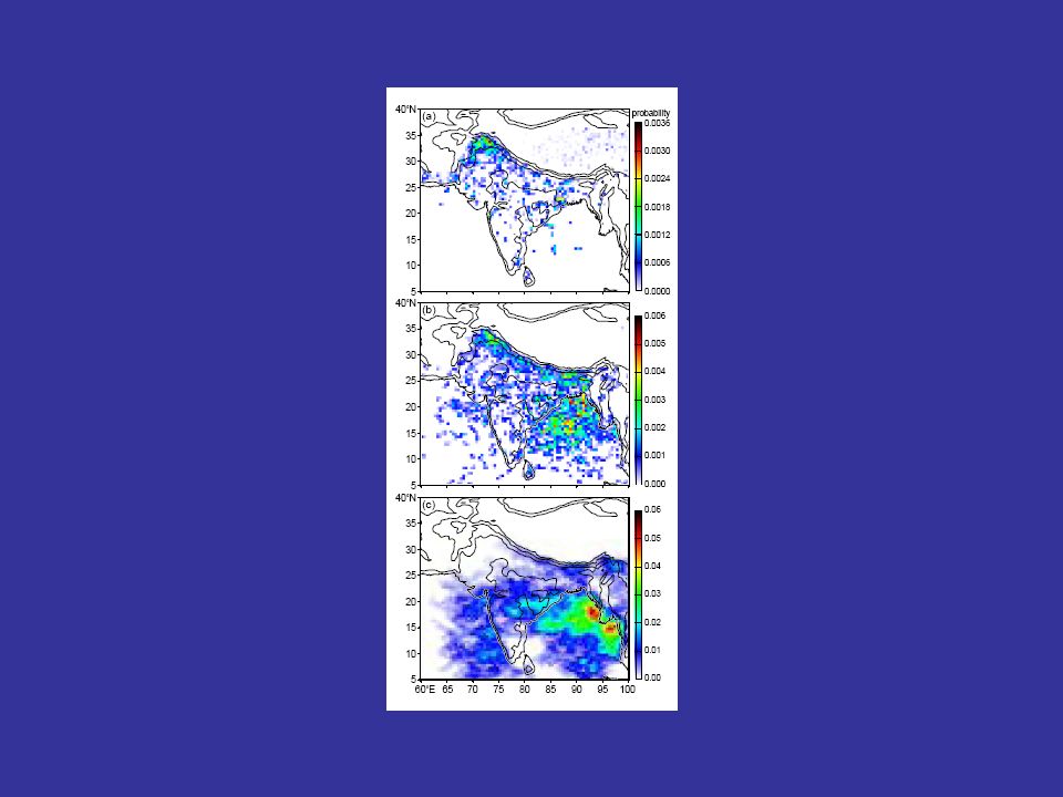
Climatología de los sistemas extremos
(de acuerdo a 8 años de datos radar de precipitación de TRMM) Distribución de la probabilidad de encontrar cada tipo de sistema Núcleos de convección profunda Regiones extensas de eco estratiforme Houze et al. (2007), Romatschke et al. (2009)
 Distribución de la probabilidad de encontrar cada tipo de sistema. Núcleos de convección profunda. Regiones extensas de eco estratiforme. Houze et al. (2007), Romatschke et al. (2009)")
43
Objetivo (parte sobre climas cálidos): 1
Objetivo (parte sobre climas cálidos): 1. Evaluar si los modelos de mesoescala de alta resolución pueden reproducir los sistemas observados 2. Investigar el efecto de la orografía en la ocurrencia y distribución espacial de cada tipo de sistema Observational studies have proposed hypotheses on how the convection forms in this region during the monsoon Our objective is to test these hypotheses (which will be explained as we go along) using model simulations
: 1. Evaluar si los modelos de mesoescala de alta resolución pueden reproducir los sistemas observados 2. Investigar el efecto de la orografía en la ocurrencia y distribución espacial de cada tipo de sistema. Observational studies have proposed hypotheses on how the convection forms in this region during the monsoon. Our objective is to test these hypotheses (which will be explained as we go along) using model simulations.")
44
Modelo y datos usados Modelo: Weather Research and Forecasting
Datos: TRMM y NCEP Resultados presentados: Región extensa de eco estratiforme observado por TRMM el 11 de agosto de 2002 The simulations were conducted with WRF, with BMP with 6 types of water categories We complemented the simulations with NCEP reanalysis Notes on simulation WRF single-moment (WSM) 6-class bulk microphysical parameterization (BMP) scheme (WSM-6, Hong et al. 2004, Hong and Lim 2006) PBL: Yonsei University (YSU) Land surface: 5-layer thermal diffusion Radiation: RRTM longwave, Dudhia shortwave Cumulus scheme: Betts-Miller-Janjic 30 vertical sigma levels Weather Research and Forecasting (WRF v2.1.1) model (runs conducted by Anil Kumar, NCAR/Purdue University) NCEP Reanalysis used as initial and boundary conditions (6 hourly) Bulk microphysical parameterization: WRF Single-Moment with 6 water substances Isolated deep convective system: dx1=9 km; dx2 = 3 km (14 Jun 2002) Simulation couldn’t capture system Wide intense convective system (3 Sep 2003) Broad stratiform system (11 Aug 2002) HYSPLIT model trajectories using NCEP reanalysis ( Wide convective: Domain 1: 180x180 grid points, time step = 60 s Domain 2: 355x334 grid points, time step = 20 s Simulation period: UTC 3 Sep 2003 Two-way nested Broad stratiform: Domain 1: 140x140 grid points, time step = 60 s Domain 2: 220x200 grid points, time step = 20 s Simulation period: 1200 UTC 10 Aug UTC 11 Aug 2002 One-way nested 44
 6-class bulk microphysical parameterization (BMP) scheme (WSM-6, Hong et al. 2004, Hong and Lim 2006) PBL: Yonsei University (YSU) Land surface: 5-layer thermal diffusion. Radiation: RRTM longwave, Dudhia shortwave. Cumulus scheme: Betts-Miller-Janjic. 30 vertical sigma levels. Weather Research and Forecasting (WRF v2.1.1) model (runs conducted by Anil Kumar, NCAR/Purdue University) NCEP Reanalysis used as initial and boundary conditions (6 hourly) Bulk microphysical parameterization: WRF Single-Moment with 6 water substances. Isolated deep convective system: dx1=9 km; dx2 = 3 km (14 Jun 2002) Simulation couldn’t capture system. Wide intense convective system (3 Sep 2003) Broad stratiform system (11 Aug 2002) HYSPLIT model trajectories using NCEP reanalysis ( Wide convective: Domain 1: 180x180 grid points, time step = 60 s. Domain 2: 355x334 grid points, time step = 20 s. Simulation period: UTC 3 Sep Two-way nested. Broad stratiform: Domain 1: 140x140 grid points, time step = 60 s. Domain 2: 220x200 grid points, time step = 20 s. Simulation period: 1200 UTC 10 Aug UTC 11 Aug One-way nested. 44.")
45
Terreno y precipitación acumulada durante la simulación
(12 UTC 10 Ago – 03 UTC 11 Ago 2002 = 18 LST 10 Ago - 09 LST 11 Ago) Domino 1: dx = 27 km Domino 2: dx = 9 km Dominio 3: dx = 3 km
 Domino 1: dx = 27 km. Domino 2: dx = 9 km. Dominio 3: dx = 3 km.")
46
Evaluation of low-levels winds at 00 UTC 11 Aug 2002
Observations 10 m winds and wind speed (m/s) WRF-simulation Surface winds and wind speed (m/s)
 WRF-simulation Surface winds and wind speed (m/s)")
47
Sounding at Tengchong at 00 UTC 11 Aug 2002
Observations WRF-simulation

48
Reflectividad instantanea (~03 UTC 11 Ago 2002)
Observations WRF-simulation Cortes horizontales a 4km Cortes verticales a lo largo de la linea negra

49
Objetivos 1. Evaluar si los modelos de mesoescala de alta resolución pueden reproducir los sistemas observados 2. Investigar el efecto de la orografía en la ocurrencia y distribución espacial de cada tipo de sistema Observational studies have proposed hypotheses on how the convection forms in this region during the monsoon Our objective is to test these hypotheses (which will be explained as we go along) using model simulations
 using model simulations.")
50
Corte vertical a lo largo de la linea roja
Periodo inicial 1415 UTC 10 Ago Periodo maduro 0130 UTC 11 Ago Reflectividad y Velocidad vertical (|1 m/s|) Hidrometeoros: Graupel: color Nieve: azul (0.1 g/kg) Lluvia: rojo (0.1 g/kg)
 Hidrometeoros: Graupel: color. Nieve: azul (0.1 g/kg) Lluvia: rojo (0.1 g/kg)")
51
Promedios temporales durante toda la simulación
Viento a 850mb Viento en superficie (11 m/s) Flujo de claro latente de la superficie (200 W/m2) Agua precipitable (67 mm) Precipitación acumulada (10 mm) Viento a 850mb Altura geopotencial a 850 mb Agua precipitable (67 mm) Flujo perpendicular a la dirección de l corte. Positivo: izq a derecha Precipitación acumulada (20 y 50 mm) Velocidad vertical a 500 mb (0.5 m/s)
 Flujo de claro latente de la superficie (200 W/m2) Agua precipitable (67 mm) Precipitación acumulada (10 mm) Viento a 850mb. Altura geopotencial a 850 mb. Agua precipitable (67 mm) Flujo perpendicular. a la dirección de l corte. Positivo: izq a derecha. Precipitación acumulada (20 y 50 mm) Velocidad vertical a 500 mb (0.5 m/s)")
52
El modela de mesoscala fue capaz de replicar el sistema observado
Conclusiones – (Precipitación estratiforme al sureste de los Himalayas) El modela de mesoscala fue capaz de replicar el sistema observado Durante la ocurrencia de estos sistemas, el flujo intenso de bajos niveles extrae eficientemente humedad de la Bahía de Bengala y de la delta del rio Ganges Cuando flujo condicionalmente inestable llega al pie de los Himalayas, es levantado sobre la topografía, alcanza la saturación y se vuelve inestable Conforme el sistema envejece, los ecos se van debilitando y se amalgaman en grandes regiones estratiformes, las cuales son a su vez sujetas a levantamiento orográfico
 El modela de mesoscala fue capaz de replicar el sistema observado. Durante la ocurrencia de estos sistemas, el flujo intenso de bajos niveles extrae eficientemente humedad de la Bahía de Bengala y de la delta del rio Ganges. Cuando flujo condicionalmente inestable llega al pie de los Himalayas, es levantado sobre la topografía, alcanza la saturación y se vuelve inestable. Conforme el sistema envejece, los ecos se van debilitando y se amalgaman en grandes regiones estratiformes, las cuales son a su vez sujetas a levantamiento orográfico.")
54
Tipo de suelo Snow/Ice Thar Desert Ganges Delta Tundra Wetland Forest
Irrigated crop Crop Savanna Shurb/Grass Dryland/crop Grass Shurb Barren Thar Desert Ganges Delta This region is interesting because it has large terrain gradients with the Indus and Ganges Plains a small distance away from the Himalayas and Hindu Kush mountains of Afghanistan We found that the land-ocean contrast between the Indian subcontinent and the Arabian Sea and Bay of Bengal was also important Also this region has strong land cover gradients, with the west side characterized by barren land (in particulat the Thar Desert) and the east side characterized by forest, irrigated crops and wetlands (in paticular Ganges Delta) 55 54
 and the east side characterized by forest, irrigated crops and wetlands (in paticular Ganges Delta)")
56
Convección profunda en los Trópicos
Altura máxima del contorno de 40 dBZ de acurdo a los datos del radar de precipitación de TRMM Following the theme on convection, I’m going to present a study on monsoon convection in the Himalayan region and in particular on how the convection is modulated by the terrain and land surface. This work was a collaboration with Robert Houze, Anil Kumar and Dev Niyogi Zipser et al. (2006) 56
 56.")
57
Convección profunda en los Trópicos
Altura máxima del contorno de 40 dBZ de acurdo a los datos del radar de precipitación de TRMM Following the theme on convection, I’m going to present a study on monsoon convection in the Himalayan region and in particular on how the convection is modulated by the terrain and land surface. This work was a collaboration with Robert Houze, Anil Kumar and Dev Niyogi Zipser et al. (2006) 57
 57.")
58
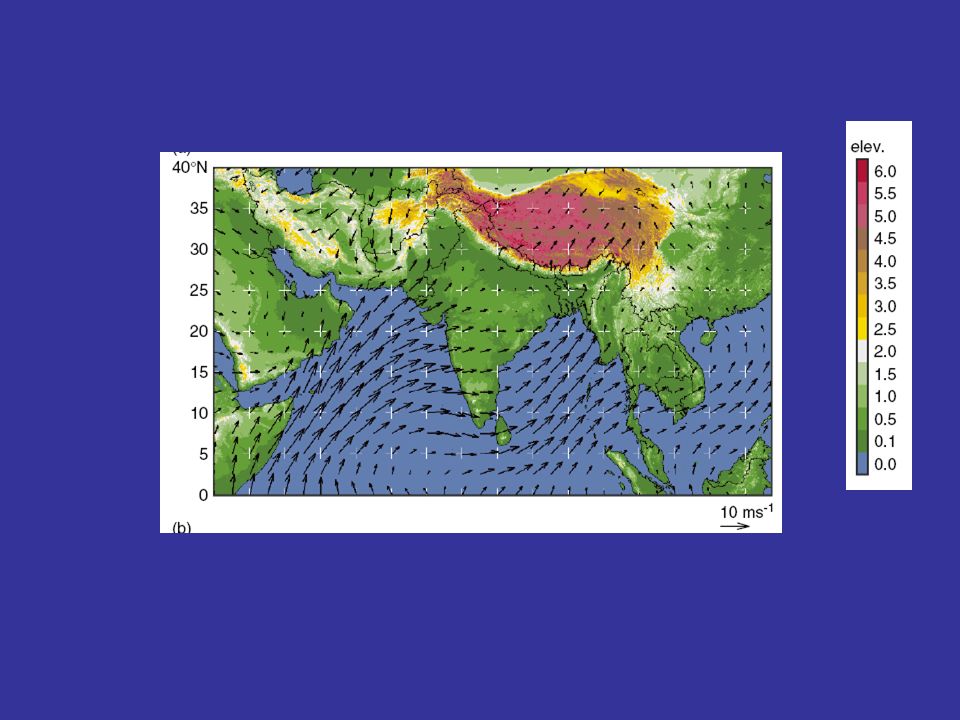
Climatología de vientos de superficie y convección profunda durante el monzón (jun-sep)
y agua precipitable (NCEP) Probabilidad de encontrar un sistema convectivo con contorno de 40 dBZ > 10 km (Radar de precipitación TRMM) Punjab Romatschke et al. (2009)
 Probabilidad de encontrar un sistema. convectivo con contorno de 40 dBZ > 10 km. (Radar de precipitación TRMM) Punjab. Romatschke et al. (2009)")
59
Los estudios de Sawyer et al. (1947) y Houze et al
Los estudios de Sawyer et al. (1947) y Houze et al. (2007) propusieron hipótesis sobre como se forma la convección profunda en la zona Objetivo (parte sobre climas cálidos): Evaluar la validez de esas hipótesis usando observaciones y simulaciones de un modelo de mesoescala Observational studies have proposed hypotheses on how the convection forms in this region during the monsoon Our objective is to test these hypotheses (which will be explained as we go along) using model simulations
 y Houze et al. (2007) propusieron hipótesis sobre como se forma la convección profunda en la zona. Objetivo (parte sobre climas cálidos): Evaluar la validez de esas hipótesis usando observaciones y simulaciones de un modelo de mesoescala. Observational studies have proposed hypotheses on how the convection forms in this region during the monsoon. Our objective is to test these hypotheses (which will be explained as we go along) using model simulations.")
60
Modelo y datos usados Modelo: Weather Research and Forecasting
Datos: TRMM y NCEP Sistema analizado: 3 sep 2003, cuando TRMM observo un sistema de convección profunda en la zona de interés The simulations were conducted with WRF, with BMP with 6 types of water categories We complemented the simulations with NCEP reanalysis Notes on simulation WRF single-moment (WSM) 6-class bulk microphysical parameterization (BMP) scheme (WSM-6, Hong et al. 2004, Hong and Lim 2006) PBL: Yonsei University (YSU) Land surface: 5-layer thermal diffusion Radiation: RRTM longwave, Dudhia shortwave Cumulus scheme: Betts-Miller-Janjic 30 vertical sigma levels Wide convective: Domain 1: 180x180 grid points, time step = 60 s Domain 2: 355x334 grid points, time step = 20 s Simulation period: UTC 3 Sep 2003 Two-way nested Broad stratiform: Domain 1: 140x140 grid points, time step = 60 s Domain 2: 220x200 grid points, time step = 20 s Simulation period: 1200 UTC 10 Aug UTC 11 Aug 2002 One-way nested 60
 6-class bulk microphysical parameterization (BMP) scheme (WSM-6, Hong et al. 2004, Hong and Lim 2006) PBL: Yonsei University (YSU) Land surface: 5-layer thermal diffusion. Radiation: RRTM longwave, Dudhia shortwave. Cumulus scheme: Betts-Miller-Janjic. 30 vertical sigma levels. Wide convective: Domain 1: 180x180 grid points, time step = 60 s. Domain 2: 355x334 grid points, time step = 20 s. Simulation period: UTC 3 Sep Two-way nested. Broad stratiform: Domain 1: 140x140 grid points, time step = 60 s. Domain 2: 220x200 grid points, time step = 20 s. Simulation period: 1200 UTC 10 Aug UTC 11 Aug One-way nested. 60.")
61
Simulación: precipitación acumulada y terreno
Dominio1 (dx = 9 km) Domino 2 (dx = 3 km) INDIA PAKISTAN HIMALAYAS HINDU KUSH This simulations was conducted with a 9km resolution domain. The terrain is shown in gray shades and show the Himalayas and Hindu Kush mountains of Afghanistan Nested within the first domain was another domain with 3 km resolution The color field shows the accumulated precipitation during the period of the simulations (which lasted 5 hours) That system occurred in the W indentation of the terrain Simulation: Started at UTC 3 Sep (5 hours) = 2300 LST 3 Sep – 0400 LST 4 Sep [LST Pakistan = UTC ]. Convection started at 1900 UTC 3 Sep = 0000 LST 4 Sep Ulli’s diurnal cycle goes form LST (night and morning systems along foothills) and (afternoon and evening systems all over the low-lands, not clustered) 61
 Domino 2 (dx = 3 km) INDIA. PAKISTAN. HIMALAYAS. HINDU KUSH. This simulations was conducted with a 9km resolution domain. The terrain is shown in gray shades and show the Himalayas and Hindu Kush mountains of Afghanistan. Nested within the first domain was another domain with 3 km resolution. The color field shows the accumulated precipitation during the period of the simulations (which lasted 5 hours) That system occurred in the W indentation of the terrain. Simulation: Started at UTC 3 Sep (5 hours) = 2300 LST 3 Sep – 0400 LST 4 Sep [LST Pakistan = UTC ]. Convection started at 1900 UTC 3 Sep = 0000 LST 4 Sep. Ulli’s diurnal cycle goes form LST (night and morning systems along foothills) and (afternoon and evening systems all over the low-lands, not clustered) 61.")
62
Evaluación: Localización del sistema respecto al terreno y temperatura del tope de la nube
(~2130 UTC 3 Sep [~0230 LST 4 Sep]) OBSERVACION SIMULACION
 OBSERVACION. SIMULACION.")
64
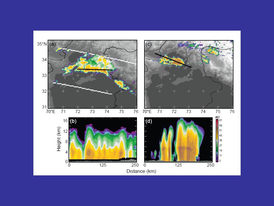
Evaluation: 3D Reflectivity structure (~22 UTC 3 Sep [~03 LST 4 Sep])
OBSERVATION (TRMM-PR) SIMULATION dBZ Horizontal cross sections at 4 km Distance (km) Height (km) Distance (km) Height (km) Vertical cross sections along black line To evaluate the simulations, we compared with several observations Here I’m just going to present the comparison with reflectivity as observed by TRMM PR An horizontal cross-section shows that the system developed more or less in the right location and that the intensity and timing was well captured In both representations the system has a strengthened and weakened parts. The apparent orientation of this line is different in the simulation from the observation (which is only a snapshot so we don’t know anything of the evolution) However the simulation did capture the two parts of the system Vertical cross-section along the strengthened parts (black line) show vertically erect convective echoes, the simulated reflectivity is slightly deeper and stronger particularly between 6-12 km Vertical cross-section along the weakened parts (red line) show a more stratiform echo, with evidence of a bright line and some embedded convection, suggesting that the collapsing convective cells are forming the stratiform echo The simulation therefore was able to depict the vertical structure of this storm so we will used the output to test the hypotheses proposed by observational studies Distance (km) Height (km) Distance (km) Height (km) Vertical cross sections along red line
![Evaluation: 3D Reflectivity structure (~22 UTC 3 Sep [~03 LST 4 Sep])](http://slideplayer.es/slide/1030849/2/images/64/Evaluation%3A+3D+Reflectivity+structure+%28%7E22+UTC+3+Sep+%5B%7E03+LST+4+Sep%5D%29.jpg "OBSERVATION (TRMM-PR) SIMULATION. dBZ. Horizontal cross. sections at 4 km Distance (km) Height (km) Distance (km) Height (km) Vertical cross. sections along. black line. To evaluate the simulations, we compared with several observations. Here I’m just going to present the comparison with reflectivity as observed by TRMM PR. An horizontal cross-section shows that the system developed more or less in the right location and that the intensity and timing was well captured. In both representations the system has a strengthened and weakened parts. The apparent orientation of this line is different in the simulation from the observation (which is only a snapshot so we don’t know anything of the evolution) However the simulation did capture the two parts of the system. Vertical cross-section along the strengthened parts (black line) show vertically erect convective echoes, the simulated reflectivity is slightly deeper and stronger particularly between 6-12 km. Vertical cross-section along the weakened parts (red line) show a more stratiform echo, with evidence of a bright line and some embedded convection, suggesting that the collapsing convective cells are forming the stratiform echo. The simulation therefore was able to depict the vertical structure of this storm so we will used the output to test the hypotheses proposed by observational studies Distance (km) Height (km) Distance (km) Height (km) Vertical cross. sections along. red line.")
65
HYPOTHESIS: Dry line SURFACE DEW POINT DEPRESSION
AND 2 AND 4 KM TERRAIN CONTOURS The first hypothesis is regarding a dry line, that is boundary or transition zone dry air from moist air. The convection formed first in the location where the bullet is an hour later We see that there is a dry line near this location Valid: 18 UTC 3 Sep (23 LST) Forecast : 0 h (1 h before convection initialization) 65
 Forecast : 0 h (1 h before convection initialization) 65.")
67
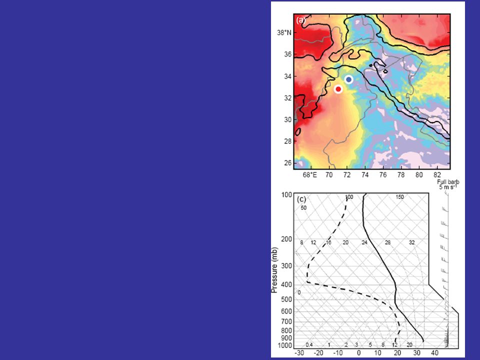
HYPOTHESIS: Moist low-level flow from Arabian Sea, dry flow aloft from Tibetan or Afghan mountains
SURFACE MIXING RATIO (g/kg) NOAA HYSPLIT (NCEP FNL) BACKWARD TRAJECTORIES 1.0 AGL km 3.5 AGL km Valid: 18 UTC 3 Sep (23 LST) Forecast : 0 h H07 hypothesized about the origin of the dry and moist flows. To investigate this, we take three points along the tongue of high mixing ration along the eastern foothills. We conduct backward trajectories using NCEP FNL analysis (since the simulation only lasted 5 hours) At 1 km AGL we see that the parcels originated from the Arabian Sea 3-4 days earlier At 3.5 km AGL they originated at the Afghan mountains. We can refine the hypothesis (at least for this cases) This is similar to the severe convection in the US Great Plains End time: 18 UTC 3 Sep (23 LST) Elapsed period between markers: 24 h 67
 NOAA HYSPLIT (NCEP FNL) BACKWARD TRAJECTORIES. 1.0 AGL km. 3.5 AGL km. Valid: 18 UTC 3 Sep (23 LST) Forecast : 0 h. H07 hypothesized about the origin of the dry and moist flows. To investigate this, we take three points along the tongue of high mixing ration along the eastern foothills. We conduct backward trajectories using NCEP FNL analysis (since the simulation only lasted 5 hours) At 1 km AGL we see that the parcels originated from the Arabian Sea 3-4 days earlier. At 3.5 km AGL they originated at the Afghan mountains. We can refine the hypothesis (at least for this cases) This is similar to the severe convection in the US Great Plains. End time: 18 UTC 3 Sep (23 LST) Elapsed period between markers: 24 h. 67.")
68
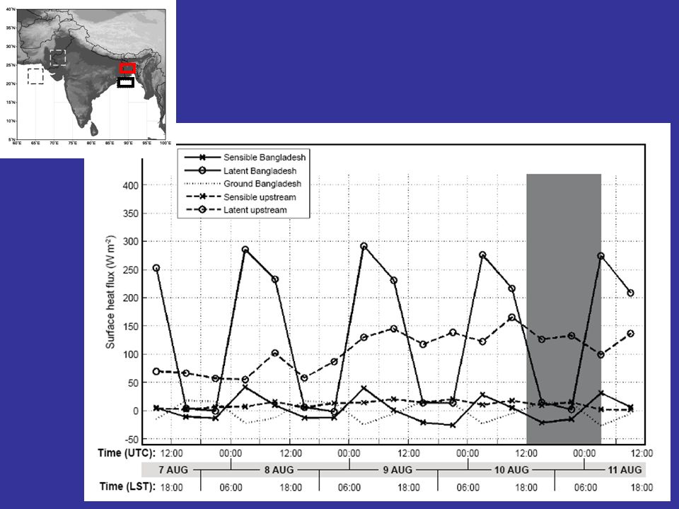
HYPOTHESIS: High surface sensible heat flux as low-level air moves over Thar Desert
NCEP time series The next hypothesis is that the flow builds up buoyancy as the low-level flow, which was moist and had high theta-e from being in contact with the Arabian Sea, is subjected to further heating by surface sensible heat flux over the Thar Desert. Fig. CASE1-FLUX: NCEP reanalysis time series of surface fluxes of sensible, latent, and ground heat (indicated by crosses, circles, and dotted line, respectively) in the days leading up to the wide convective system event of 2200 UTC 03 Sep The fluxes averaged over the Thar Desert (25-29°N and 69-73°E, long dashed white rectangle in Fig. SYSTEMS) are shown by the solid and dotted lines. The fluxes averaged immediately upstream of the Thar Desert, over the Arabian Sea (20-24°N and 63-67°E, long dashed black rectangle in Fig. SYSTEMS)
 in the days leading up to the wide convective system event of 2200 UTC 03 Sep The fluxes averaged over the Thar Desert (25-29°N and 69-73°E, long dashed white rectangle in Fig. SYSTEMS) are shown by the solid and dotted lines. The fluxes averaged immediately upstream of the Thar Desert, over the Arabian Sea (20-24°N and 63-67°E, long dashed black rectangle in Fig. SYSTEMS)")
69
Land cover Snow/Ice Thar Desert Tundra Wetland Forest Irrigated crop
Savanna Shurb/Grass Dryland/crop Grass Shurb Barren Thar Desert This region is interesting because it has large terrain gradients with the Indus and Ganges Plains a small distance away from the Himalayas and Hindu Kush mountains of Afghanistan We found that the land-ocean contrast between the Indian subcontinent and the Arabian Sea and Bay of Bengal was also important Also this region has strong land cover gradients, with the west side characterized by barren land (in particulat the Thar Desert) and the east side characterized by forest, irrigated crops and wetlands (in paticular Ganges Delta) 55 69
 and the east side characterized by forest, irrigated crops and wetlands (in paticular Ganges Delta)")
70
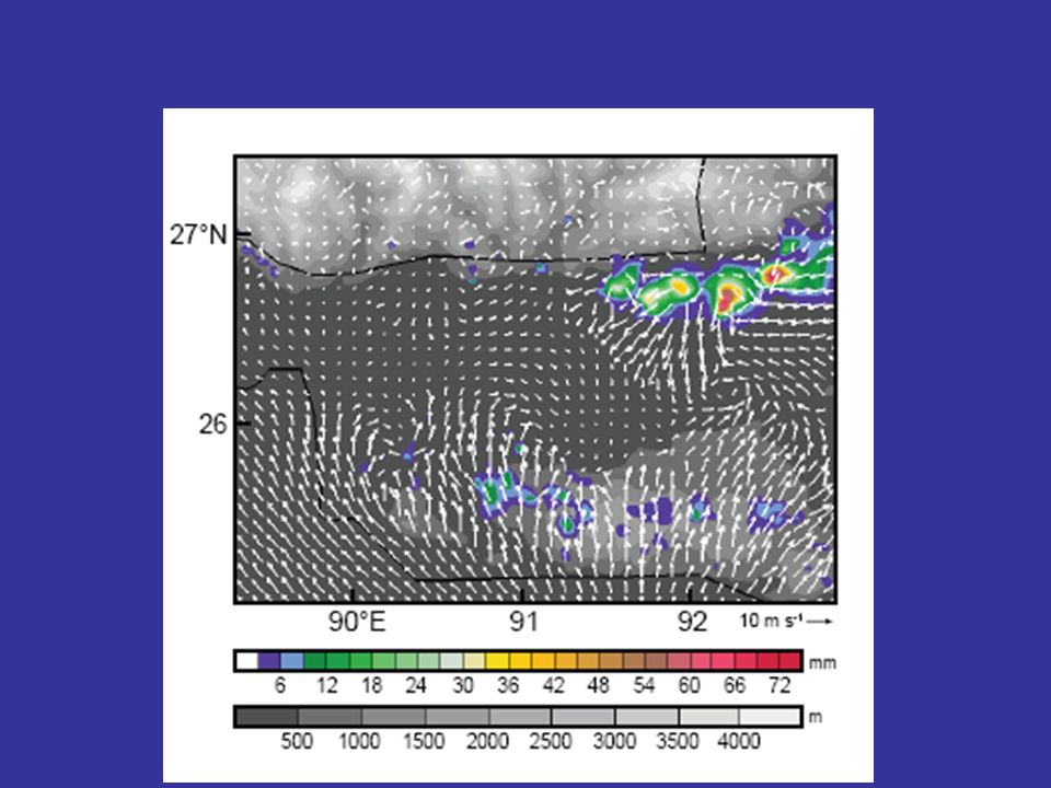
HYPOTHESIS: Convection triggered over foothills
TERRAIN AND COLUMN INTEGRATED PRECIPITATION HYDROMETEORS (10 mm) TOTAL PRECIP. MIXING RATIO N 6.0 g kg-1 Valid: 19 UTC 3 Sep (00 LST). Forecast : 1 h 70
 TOTAL PRECIP. MIXING RATIO. N. 6.0 g kg-1. Valid: 19 UTC 3 Sep (00 LST). Forecast : 1 h. 70.")
71
dry,hot moist Carlson et al. 1983
Therefore they suggested that something similar to what happens in the US plains is occurring. In the US plains there a layer of dry flow that originates over an elevated plateau to the west that heats up during the day by being in contact with the terrain. This layer caps moist air that has its origin over the Gulf of Mexico According to Carlson, intense convection may occasionally break through the lid or break out along the lid edge.

72
Conclusiones – (Convección profunda en Punjab)
El flujo del aire a niveles bajos obtiene humedad del Mar Arábigo y es calentado por su paso por del desierto del Thar Una capa elevada de aire seco y cálido proveniente de la región de Afganistán esta localizado sobre el aire húmedo cerca de la superficie y retarda el inicio de la convección La convección es eventualmente detonada por forzamiento orográfico sobre los picos pequeños

77
Reflectividad (promedio de 3 h)
MAP IOP2b Reflectividad (promedio de 3 h) dBZ Tipo A 1. Mean reflectivity for the same cross sections shown before for Type A cases show convective-like echo structure over the 1st major peak of the terrain. 2. As the low stability flow rises over the terrain, low-level moisture is transported over the first peak of the terrain. In addition, the slight instability of the flow is released on the upslope flow contributing to this convective signature. NNW RADAR
 dBZ. Tipo A. 1. Mean reflectivity for the same cross sections shown before for Type A cases show convective-like echo structure over the. 1st major peak of the terrain. 2. As the low stability flow rises over the terrain, low-level moisture is transported over the first peak of the terrain. In addition, the slight instability of the flow is released on the upslope flow contributing to this convective signature. NNW. RADAR.")
78
Reflectividad (promedio de 3 h)
MAP IOP3 Reflectividad (promedio de 3 h) dBZ Tipo A 1.We see the same structure for the other two Type A cases. NNW RADAR
 dBZ. Tipo A. 1.We see the same structure for the other two Type A cases. NNW. RADAR.")
79
Particle Type Frequency (%)
MAP IOP2b Particle Type Frequency (%) Graupel Tipo A Dry snow Melting snow 1.This cross-section shows accumulated frequency of occurrence of particle types as derived from S-pol radar data during IOP2b. 2. Graupel (indicated by the color shading) occurred preferentially above the first peak of the terrain, directly above the reflectivity maximum, implying that riming was also important to the growth of precipitation on the windward slopes. 4.The intermittent graupel occurred as a result of the release of instability and it was embedded in a broad layer of dry snow (cyan) which was melting and falling into a layer of wet snow (orange). Dry snow: 45% Wet snow: 30 % NNW RADAR
 Graupel. Tipo A. Dry snow. Melting snow. 1.This cross-section shows accumulated frequency of occurrence of particle types as derived from S-pol radar data during IOP2b. 2. Graupel (indicated by the color shading) occurred preferentially above the first peak of the terrain, directly above the reflectivity maximum, implying that riming was also important to the growth of precipitation on the windward slopes. 4.The intermittent graupel occurred as a result of the release of instability and it was embedded in a broad layer of dry snow (cyan) which was melting and falling into a layer of wet snow (orange). Dry snow: 45% Wet snow: 30 % NNW. RADAR.")
80
Particle Type Frequency (%)
MAP IOP3 Particle Type Frequency (%) Graupel Tipo A Dry snow Melting snow 1.The same distribution of hydrometeors was observed during the other two Type A cases Dry snow: 30% Wet snow: 5% NNW RADAR
 Graupel. Tipo A. Dry snow. Melting snow. 1.The same distribution of hydrometeors was observed during the other two Type A cases. Dry snow: 30% Wet snow: 5% NNW. RADAR.")
81
Reflectividad (promedio de 3 h)
IMPROVE-2 Case 11 Reflectividad (promedio de 3 h) dBZ Tipo B 1.The same was observed during the other two Type B cases. 2.A secundary maximum of reflectivity around km was also observed. 3.This secundary maximum was seen at ~-13deg C, so one hypothesis for its formation is the aggregation of dendrites that is likely to occur at this temperature. RADAR E
 dBZ. Tipo B. 1.The same was observed during the other two Type B cases. 2.A secundary maximum of reflectivity around km was also observed. 3.This secundary maximum was seen at ~-13deg C, so one hypothesis for its formation is the aggregation of dendrites that is likely to occur at this temperature. RADAR. E.")
82
3-hour Mean Radial velocity
IMPROVE-2 Case 1 3-hour Mean Radial velocity dBZ Tipo B RADAR E

83
Particle Type Frequency (%)
IMPROVE-2 Case 11 Particle Type Frequency (%) Graupel/ aggregates Tipo B Dry snow Melting snow 1.The other two Type B cases had similar structure Dry snow: 70% Wet snow: 40% RADAR E
 Graupel/ aggregates. Tipo B. Dry snow. Melting snow. 1.The other two Type B cases had similar structure. Dry snow: 70% Wet snow: 40% RADAR. E.")
84
Particle Type Frequency (%)
IMPROVE-2 Case 1 Particle Type Frequency (%) Graupel/ aggregates Tipo B Dry snow Melting snow Dry snow: 45% Wet snow: 35% RADAR E
 Graupel/ aggregates. Tipo B. Dry snow. Melting snow. Dry snow: 45% Wet snow: 35% RADAR. E.")
85
Vertically pointing radar
IMPROVE-2 Case 11 – Type B Vertically pointing radar Similar VP updrafts were observed in a different mountain range in the other two Type B cases. So how were these updraft cells created?

86
Vertically pointing radar
IMPROVE-2 Case 1 – Type B Vertically pointing radar

87
IMPROVE-2 Case 1 – KH billows

88
Terrain gradients Land-ocean contrast Land cover gradients
Snow/Ice Tundra Wetland Forest Irrigated crop Crop Savanna Shurb/Grass Dryland/crop Grass Shurb Barren Thar Desert Ganges Delta This region is interesting because it has large terrain gradients with the Indus and Ganges Plains a small distance away from the Himalayas and Hindu Kush mountains of Afghanistan We found that the land-ocean contrast between the Indian subcontinent and the Arabian Sea and Bay of Bengal was also important Also this region has strong land cover gradients, with the west side characterized by barren land (in particulat the Thar Desert) and the east side characterized by forest, irrigated crops and wetlands (in paticular Ganges Delta) 55 88
 and the east side characterized by forest, irrigated crops and wetlands (in paticular Ganges Delta)")
89
Durante el monzón (jun-sep), cuando los vientos en superficie son del suroeste, la convección profunda se concentra en la identacion Sistemas de convección profunda

92
Distribución geográfica de los sistemas convectivos de acuerdo al radar de precipitación de TRMM
Houze et al. (2007)
")
93
Relación entre los procesos microfisicos/corrientes verticales y la estructura vertical de la precipitación Houze (1997)
")
94
Example of Broad Stratiform Echo
(>50,000 km2 in area) 00 UTC 11 Aug 2002 Tengchong sounding Example: Infrared satellite temperature and reflectivity at ~03 UTC 11 Aug 2002 10 m winds reanalysis at 00 UTC 11 Aug 2002 And when they look at a typical example, that is what they see. A cross-section thru the system shows a BB, indicating stratiform precipitation, which is often the case in maritime tropical rain (Schumacher and Houze 2003a:strat rain J Clim). The echo has evidence of weakened convective cells, suggesting that deep active cells collapsed into stratiform echo. Houze et al 2007 found that these cases often occur in conjuction with BoB monsoon depression The atmosphere is moist adiabatic throughtout Houze et al suggested that in these cases the convection was formed by a combination of widespread upward motion associated with BoB depression AND by the flow rising over the terrain IN NOT SURE ABOUT TIME IN WIND, could also be 12 UTC, check CHECK MAP IN REFERENCE Houze et al. (2007)
 00 UTC 11 Aug Tengchong sounding. Example: Infrared satellite temperature. and reflectivity at ~03 UTC 11 Aug m winds reanalysis at. 00 UTC 11 Aug And when they look at a typical example, that is what they see. A cross-section thru the system shows a BB, indicating stratiform precipitation, which is often the case in maritime tropical rain (Schumacher and Houze 2003a:strat rain J Clim). The echo has evidence of weakened convective cells, suggesting that deep active cells collapsed into stratiform echo. Houze et al 2007 found that these cases often occur in conjuction with BoB monsoon depression. The atmosphere is moist adiabatic throughtout. Houze et al suggested that in these cases the convection was formed by a combination of widespread upward motion associated with BoB depression AND by the flow rising over the terrain. IN NOT SURE ABOUT TIME IN WIND, could also be 12 UTC, check. CHECK MAP IN REFERENCE. Houze et al. (2007)")
Presentaciones similares


>")


