INTA-Instituto de Clima y Agua (Argentina)

Presentación del tema: "INTA-Instituto de Clima y Agua (Argentina)"— Transcripción de la presentación:

1 INTA-Instituto de Clima y Agua (Argentina)
Taller de Trabajo sobre Vulnerabilidad y Adaptacion Impactos, Vulnerabilidad y Adaptacion en el sector Agricola – Parte 2 Asunción Paraguay. August 14-18, 2006 Full references can be found in Chapter 11, Bibliography, of the Handbook. Graciela O. Magrin INTA-Instituto de Clima y Agua (Argentina)

2 FAOCLIM

3 Precipitacion Anual 1901-1995 Source of data: NOAA, NCDC
Precipitation changes over the last decades are more difficult to interpret than temperature changes. The slide shows precipitation changes derived form a the NOAA dataset globally and for a location in Argentina. The location is shown to highlight the large year-to-year variability of precipitation. Source of data: NOAA, NCDC. Source of data: NOAA, NCDC

4 Clasificacion de cobertura de la tierra
Eva et al., 2004 Land cover is important for agricultural studies, especially if the future adaptations include expansion of crop production areas. The figure shows a global land cover classification. Source: DeFries et al., 1998. De Fries et al., 1998 1: Evergreen needle leaf forests 2: Evergreen broad leaf forests 3: Deciduous needle leaf forests 4: Deciduous broad leaf forests 5: Mixed forests 6: Woodlands 7: Wooded grasslands/shrubs 8: Closed bushlands or shrublands 9: Open shrublands 10: Grasses 11: Croplands 12: Bare 13: Mosses and lichens

5 Poblacion Population is a key variable for evaluating social conditions in the future. The figure shows the current population map elaborated by CIESIN. Future population datasets are also available. Source:

6 La iluminacion se relaciona con la poblacion y los ingresos
Other datasets available may be interesting for evaluating social and economic conditions essential for geographically explicit studies. For example, the night-time city lights of the world are correlated to income and population. Source: DMSP (NASA and NOAA) Map of the night-time city lights of the world DMSP: NASA and NOAA

7 Suelos: FAO

8 Climate change scenarios can be obtained from the IPCC
Climate change scenarios can be obtained from the IPCC. The figure shows as examples maps of climate change scenarios constructed with the data provided by the IPCC. Source of data: IPCC; Cambios proyectados en temperatura y precipitacion annual para el 2050 en relacion con las condiciones actuales segun dos MGC.

9 Aplicaciones practicas: DSSAT
Pregunta: Que componentes del sistema agricola son mas vulnerables y requieren especial atencion? – modelos de cultivos (p.e. DSSAT) International Consortium for Agricultural Systems Applications Question 1: What components of the farming system are particularly vulnerable, and may thus require special attention? Some practical applications with crop models help contribute to answer this question. The training examples are with the DSSAT models, although other models such as WOFOST, EPIC, etc., are equally useful.

10 Aplicaciones practicas: DSSAT
Ejemplos de uso Uso de modelos (3 aplicaciones para realizar por los participantes)

11 DSSAT Decision Support System for Agrotechnology Transfer
Componentes Descripcion Base de Datos Clima, Suelo, Genetico, experimentos, economica Modelos Modelos de cultivos: maiz, trigo, arroz, cebada, sorgo, soja, mani, papa, etc) Programas Graficos, clima, coeficientes geneticos, suelos, etc Aplicaciones Validacion, analisis de sensibilidad estrategias estacionales, rotacion de cultivos

12 Datos Requeridos Clima: Valores diarios de precipitacion, temperatura maxima y minima y radiacion Suelos: Textura y contenido de humedad Manejo: fecha y densidad de siembra, variedad, espaciamiento, riego y fertilizacion (fecha y monto). Datos de cultivo: fechas de floracion y madurez, materia seca y rendimiento, medidas de crecimiento y area foliar.

13 Validacion del modelo Trigo: 23 sitios (m.e.: 10%)
Soja: 16 sitios (m.e.: 10.9% Maiz: 11 sitios ( m.e.: 7.8% Validacion del modelo Travasso & Magrin, 2001

14 Ejemplos Un manejo optimo del cultivo puede ser una opcion de adaptacion? Puede lograrse la adaptacion optimizando los cultivares? El cambio en la mezcla de cultivods puede ser una adaptacion? The following examples illustrate the results of the application of crop models for encouraging participants to test similar examples during the PC-based training.

15 Un manejo optimo del cultivo puede ser una opcion de adaptacion?
Source Argentina 2º National communication Source: Muchena, 1994.

16 Un manejo optimo del cultivo puede ser una opcion de adaptacion?
Estrategias de adaptacion en 2 sitios de Argentina Incrementar insumos y mejorar el manejo: Fecha de bsiembra Fertilizacion Riego suplementario Source: Muchena, 1994. Travasso et al., 2006

17 Crop Coefficients Corn
Puede lograrse la adaptacion optimizando los cultivares? . Fase Juvenil (grados dia sobre 8C desde esmergencia hasta fin de la fase juvenil) . Sensibilidad a Fotoperiodo . Duracion de llenado de granos (grados dia sobre 8C desde floracion hasta madurez) . Numero potencial de gtranos . Peso potencial de granos (tasa de crecimiento) P1 P2 P5 G2 G5 The coefficients that define crop varieties in the model can represent the characteristic of “hypothetical” future varieties. The models may assist in the development of new varieties more adapted to the climate change conditions. In the DSSAT models, the coefficients that describe a particular crop variety are included in a file of “genetic coefficients” that conceptually represent each crop variety.

18 Optimizacion de variedades
Maiz >P1 Prolongacion de la Fase juvenil Trigo >P1D mayor sensibilidad al fotoperiodo Wheat: The use of a cultivar with higher sensitivity to photoperiod would allow for an increase in the growing season duration, contributing to an increase in biomass yield. Maize: Some changes in cultivar characteristics could be done to achieve an increase in the length of the growing season effectively translated into higher production levels. Nevertheless, no changes in yield were found by changing photoperiod sensitivity (P2) and only in some cases did increases in the length of the juvenile phase (P1) translate into yield increases. (Magrin et al., 2002).

19 Aplicaciones practicas
Efectos del manejo (nitrogeno y riego suplementario) en dos zonas de Argentina Efectosn delo cambio climatico en diferentes zonas Analisis de sensibilidada a cambios en lluvia, temperatura y niveles de CO2 levels Adaptacion: Cambios en manejo para mejorar los rendimientos bajo cambio climatico. The participants now use the models installed in their PCs.

20 Aplicacion 1. Manejo The first application involves the effect of changes in crop management. The example illustrates simulated crop response in Florida (wet site) and in Syria (very dry site).

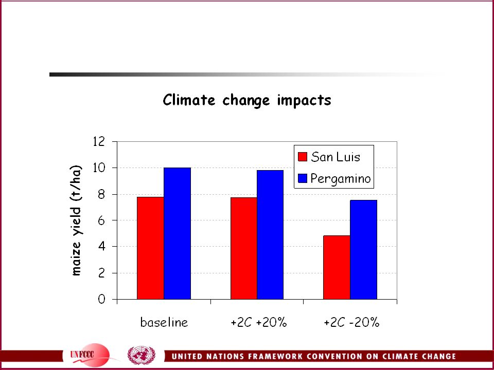
21 Clima San Luis Pergamino SR (MJ m2 day1) 17.5 15.9 T Max (°C) 24.4
22.9 T Min (°C) 11.6 10.6 Precipitacion (mm) 603 1029 Dias con lluvia (num) 65 85.4 The table summarizes the average climate in Syria and Florida, highlighting the differences in temperature and rainfall.

22 Datos de entrada necesarios
Clima Suelos Cultivares Manejo (*.MZX files) descripcion del experimento The CERES-Maize model uses several input files.

23 Abriendo DSSAT . . . First, click on the DSSAT program installed in the PC to open the program. This first screen shows the components of the DSSAT software: Data, Models, Analyses, Tools, and Options to set up the interface with other software programs (for example, excel). The weather, soil, and genotype files are under “DATA.”

24 Archivos de entrada Clima Suelo Cultivares
Examine the data files provided in the example. These data files can be used as inputs for the experiment with the crop model. Cultivares

25 Archivo de Cultivares

26 Seleccionando elcultivar. .
The cultivar file for the maize mode is MZCER980.CUL.

27 Mirando las caracteristicas del cultivar . . .
Under DATA examine the cultivar file; the screen shows the top of the cultivar file.

28 Archivos de clima . . .

29 Elegimos el clima. . .

30 Miramos los datos de clima. . .

31 Calculamos medias mensuales…..
Calculate monthly means of weather variables.

32 Calculo de medias mensuales . . . (cont…)
Result of the calculation of monthly means.

33 Ubicacion de los datos del experimento . . .
Under models, select cereals, maize, and then the input experiment file. These file included the parameters that define the agricultural experiment.

34 Seleccion del Experimento. . .

35 Archivo de Experimentos
Under experiment files, examine the experiment specifications: the soil where the crop is planted, the weather of the site where the crop is grown, the particular crop variety, and the management conditions. The slide shows the top of the file that describes the experiment in Syria.

36 Archivo de Experimentos
Under experiment files, examine the experiment specifications. The slide shows the top of the file that describes the experiment in Florida.

37 Comienzo de la simulacion….
Once the experiment is defined (soils, weather, cultivars, and management) start the simulation by clicking on “simulate.”

38 Corriendo . . . After clicking on “simulate,” the model starts running.

39 Seleccion del Experimento . . .
Select first the Florida experiment and, after completing the simulation, select the Syria experiment.

40 Selecion del Tratamiento . . .
Select the “treatment” (that is the name given in the model to each of the management alternatives) Select run all treatments.

41 Vista de los resultados . . .
The results can be viewed or the OUTPUT files can be exported to be analyzed with another program (for example, Excel).

42 Select Option . . .

43 Analis de Resultados

44 Analisis de Resultados

45 Analisis de Resultados

46 Analisis de Resultados

47 Ejemplo 2. Sensibilidad al clima
The second application shows the effect of changes in weather. The example illustrates the contrasting effects of changes in temperature and precipitation in Florida (wet site) and in Syria (very dry site). The input weather files will be modified in the “sensitivity” mode of the crop model.

48 Comienzo de la simulacion . .
Start simulation as before.

49 Analisis de sensibilidad . . .
At the screen asking whether to “run simulation” or “select sensitivity analysis options,” choose the latter.

50 Seleccion de la opcion…
Select option to be modified: Weather. Select decrease in precipitation by -50%. Continue as in the first experiment and after completing the simulation, retrieve the OUTPUT files to examine the results.

51

52 Cambios en oferta/demanda de agua. Modelos de riego suplementario (e.g., CROPWAT)
CROPWAT es us sistema de decision para el planeamiento y manejo del riego. Question 2: Can the water/irrigation systems meet the stress of changes in water supply/demand? Some practical applications with the FAO CROPWAT irrigation model will help answer this question. The training examples are with the CROPWAT model, although other models such may be equally useful.

53 Ejemplos Calculo de la ET0 Calculo de los requerimientos del cultivo
Calculo de requerimientos de riego para varios cultivos CROPWAT is used here to calculate ET0, crop water requirements, and irrigation requirements for several crops in a farm.

54 Comenzando con CROPWAT …

55 Rescatar datos de clima. .

56 Analizar Temperature . . .

57 Analizar ET0 . . . Examine ETP . . .
Alternatively, the ETP can be calculated by a range of methods included in the model.

58 Calcular ET

59 Analizar Lluvias . . .

60 Rescatar parametros del cultivo . . .

61 Ver los datos cargados . . .

62 Definir y ver areas de cultivos. . .

63 Definir el metodo de riego. . .

64 Datos de entrada completados . . .
Review that the input data are completed to start simulation.

65 Calculo de Necesidades de riego . . .

66 Calculo de Esquema de riego . . .

67 Resumen de Resultados . . .